Convolutional Neural Networks (CNN)

Introduction

Convolutional Neural Networks (CNNs) are a class of deep neural networks that are primarily used to analyze visual imagery. They employ a mathematical operation known as convolution and have proven extremely effective for various image and video recognition, recommender systems, image classification, medical image analysis, and natural language processing tasks.

Background and Theory

Convolutional Layers

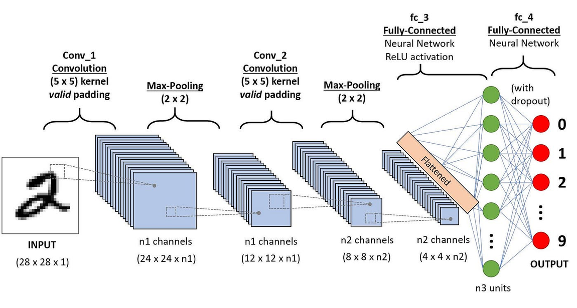
The core building block of a CNN is the convolutional layer that applies a convolution operation to the input passing the result to the next layer. Mathematically, a convolution is a combined integration of two functions and expresses how the shape of one is modified by the other. In the context of a CNN, it's used to blend the input image with a filter (or kernel) to extract features such as edges:

Here, $I$ is the input image and $K$ is the kernel. The output $S$ is known as the feature map.

Activation Functions

Following convolution, an activation function like ReLU (Rectified Linear Unit) is applied to introduce non-linearity into the model, allowing it to learn more complex patterns. ReLU is defined as:

Pooling Layers

Pooling (or subsampling or downsampling) reduces the dimensionality of each feature map but retains the most important information. Max pooling, for example, outputs the maximum value of the portion of the image covered by the kernel, a simple way to down-sample the input:

where $W_{ij}$ is the window and $X_{ab}$ are the elements of the input feature map within that window.

Fully Connected Layers

Finally, CNNs end with fully connected layers where neurons have full connections to all activations in the previous layer, as seen in regular Neural Networks. Their outputs are computed via matrix multiplication with the input and a bias offset:

Backpropagation and Training

Forward Pass

In the forward pass, each convolutional, activation, and pooling layer processes the input and passes it to the next layer. The final output is obtained after the fully connected layer.

Backpropagation

During backpropagation, the network adjusts its parameters proportionally to the error in its predictions. The process involves:

1. Loss Function Calculation: Compute the loss, which measures the prediction error. Common loss functions include mean squared error for regression tasks and cross-entropy loss for classification tasks.

2. Gradient Calculation: Use the chain rule to recursively calculate the derivatives of the loss function with respect to each weight in the network, moving backward from the output layer to the input layer.

   • For weight $w_{ij}$ in layer $l$, the gradient is:
     $\frac{\partial \mathcal{L}}{\partial w_{ij}^l} = \frac{\partial \mathcal{L}}{\partial y^l} \cdot \frac{\partial y^l}{\partial w_{ij}^l}$
   • Where $\mathcal{L}$ is the loss, and $y^l$ is the output of layer $l$.

3. Parameter Update: Update the weights using a learning rate $\eta$. A typical update rule is:

   $w_{ij}^l = w_{ij}^l - \eta \cdot \frac{\partial \mathcal{L}}{\partial w_{ij}^l}$

4. Iteration: Repeat the forward and backward pass for each batch of training data until the network performs satisfactorily.

Implementation

Structure

ConvBlock2D $\cdots$ -> Flatten -> DenseBlock $\cdots$ -> Dense

Parameters

• in_channels_list: list[int] int
  List of input channels for convolutional blocks
  
• in_features_list: list[int] int
  List of input features for dense blocks
  
• out_channels: int
  Output channels for the last convolutional layer
  
• out_features: int
  Output features for the last dense layer
  
• filter_size: int
  Size of filters for convolution layers
  
• activation: Activation
  Type of activation function
  
• optimizer: Optimizer
  Type of optimizer for weight update
  
• loss: Loss
  Type of loss function
  
• initializer: InitStr, default = None
  Type of weight initializer (None for dense layers)
  
• padding: Literal['same', 'valid'], default = ‘same’
  Padding strategy (default ‘same’)
  
• stride: int, default = 1
  Step size of filters during convolution
  
• do_batch_norm: bool, default = True
  Whether to perform batch normalization (default True)
  
• momentum: float, default = 0.9
  Momentum for batch normalization
  
• do_pooling: bool, default = True
  Whether to perform pooling
  
• pool_filter_size: int, default = 2
  Size of filters for pooling layers
  
• pool_stride: int, default = 2
  Step size of filters during pooling
  
• pool_mode: Literal['max', 'avg'], default = ‘max’
  Pooling strategy (default ‘max’)
  
• do_dropout: bool, default = True
  Whether to perform dropout
  
• dropout_rate: float, default = 0.5
  Dropout rate
  
• batch_size: int, default = 100
  Size of a single mini-batch
  
• n_epochs: int, default = 100
  Number of epochs for training
  
• learning_rate: float, default = 0.001
  Step size during optimization process
  
• valid_size: float, default = 0.1
  Fractional size of validation set
  
• lambda_: float, default = 0.0
  L2 regularization strength
  
• early_stopping: bool, default = False
  Whether to early-stop the training when the valid score stagnates
  
• patience: int, default = 10
  Number of epochs to wait until early-stopping
  
• shuffle: bool, default = True
  Whethter to shuffle the data at the beginning of every epoch

Applications

CNNs are applied in numerous domains including:

• Image and Video Recognition: Automated driving, medical imaging.
• Natural Language Processing: Sentence classification, machine translation.
• Recommendation Systems: Personalizing content based on user behavior and preferences.

Discussion on Strengths and Limitations

Strengths

• Feature Learning: CNNs automatically detect the important features without any human supervision.
• Translation Invariance: Once trained, CNNs can recognize objects in an image, regardless of where they appear.

Limitations

• High Computational Cost: Training can be computationally intensive due to the complex architectures.
• Prone to Overfitting: Especially when training data is limited.

Advanced Topics

• Deep Residual Networks: Introduce a shortcut connection that skips one or more layers.
• Dilated Convolutions: Allows the network to have a wider field of view.

References

1. LeCun, Yann, et al. "Gradient-based learning applied to document recognition." Proceedings of the IEEE, 86.11 (1998): 2278-2324.
2. Krizhevsky, Alex, Ilya Sutskever, and Geoffrey E. Hinton. "ImageNet classification with deep convolutional neural networks." NIPS. 2012.
3. Goodfellow, Ian, Yoshua Bengio, and Aaron Courville. "Deep Learning." MIT Press, 2016. link