Multi-Layer Perceptron (MLP)

Introduction

A Multilayer Perceptron (MLP) is a class of feedforward artificial neural network (ANN) that consists of at least three layers of nodes: an input layer, one or more hidden layers, and an output layer. Unlike single-layer perceptrons, MLPs can approximate complex nonlinear functions, making them powerful tools for classification and regression tasks in machine learning. The capability of MLPs to learn from data and improve their accuracy over time is facilitated by their use of backpropagation for training.

Background and Theory

Mathematical Foundations

An MLP is fundamentally composed of multiple layers of neurons, each linked by weights and biases. The architecture includes:

• Input Layer: Receives the input features.
• Hidden Layers: Intermediate layers that transform inputs into something that the output layer can use.
• Output Layer: Produces the final prediction or classification.

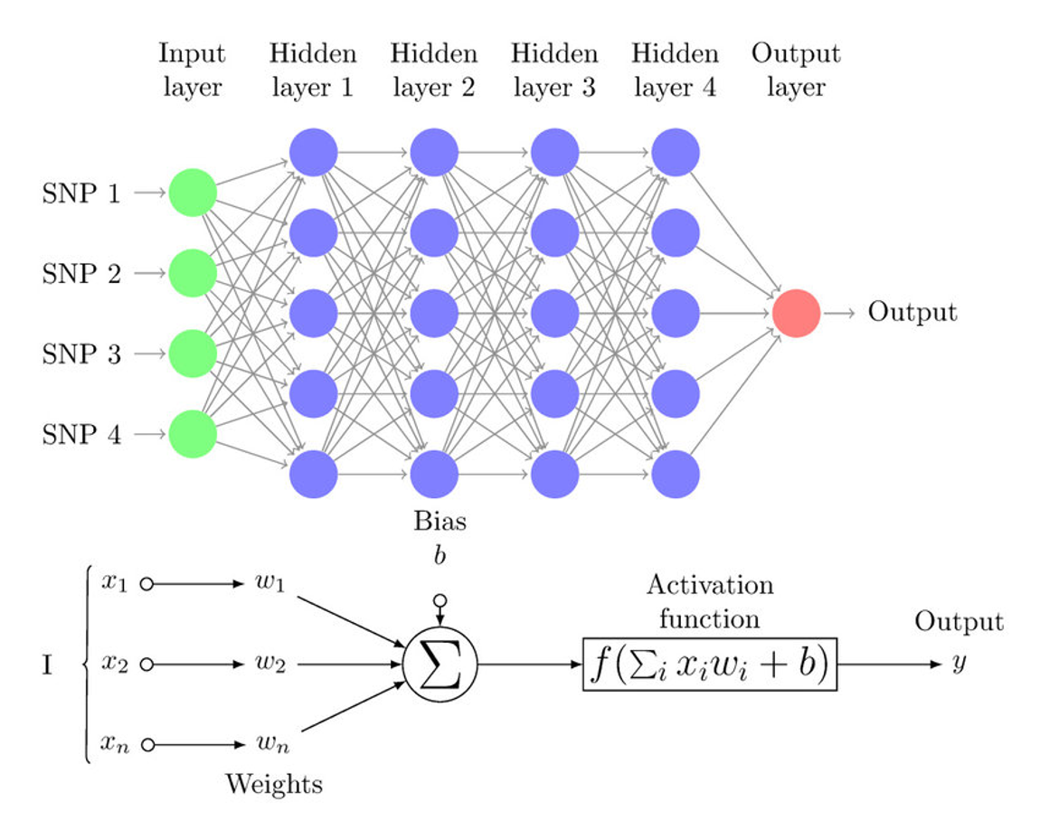
Each neuron in these layers, except for those in the input layer, uses a nonlinear activation function, which is essential for learning complex data patterns. Common activation functions include Sigmoid, Tanh, and ReLU (Rectified Linear Unit).

Forward Propagation

The process of computing the output of an MLP is called forward propagation. Given an input vector $\mathbf{x}$, the network processes this vector through each layer to produce an output. The operations in each layer $l$ can be described as follows:

1. Linear Transformation: Each neuron receives inputs from all neurons in the previous layer, multiplied by the respective weights, and summed together along with a bias term. Mathematically, this can be expressed as:

   $\mathbf{z}^{(l)} = \mathbf{W}^{(l)}\mathbf{a}^{(l-1)} + \mathbf{b}^{(l)}$

   where $\mathbf{W}^{(l)}$ and $\mathbf{b}^{(l)}$ are the weight matrix and bias vector for layer $l$, and $\mathbf{a}^{(l-1)}$ is the output vector from the previous layer (with $\mathbf{a}^{(0)} = \mathbf{x}$ for the input layer).

2. Activation Function: The linearly transformed data $\mathbf{z}^{(l)}$ is passed through a nonlinear activation function $\sigma$:

   $\mathbf{a}^{(l)} = \sigma(\mathbf{z}^{(l)})$

   This step is critical as it introduces non-linearity into the model, enabling it to learn more complex patterns.

Backward Propagation (Backpropagation)

Backpropagation is the method used to update the weights and biases of the MLP based on the error in the output. This process involves several key steps:

1. Error Calculation: Compute the loss (error) at the output, typically using a loss function, depending on the task (e.g., mean squared error for regression, cross-entropy loss for classification).

   $L = \text{Loss}(\mathbf{y}, \mathbf{\hat{y}})$

   where $\mathbf{y}$ is the true label and $\mathbf{\hat{y}}$ is the predicted output.

2. Gradient Calculation: Compute the gradients of the loss function with respect to each weight and bias in the network. This is done using the chain rule of calculus. For the output layer, the gradient of the weights is given by:

   $\frac{\partial L}{\partial \mathbf{W}^{(L)}} = \frac{\partial L}{\partial \mathbf{a}^{(L)}} \frac{\partial \mathbf{a}^{(L)}}{\partial \mathbf{z}^{(L)}} \frac{\partial \mathbf{z}^{(L)}}{\partial \mathbf{W}^{(L)}}$

   where $L$ denotes the last layer. This process is repeated recursively for each layer back to the input.

3. Update Weights and Biases: Update the weights and biases using the gradients computed and a learning rate $\eta$. The updates typically follow the rule:

   $\mathbf{W}^{(l)} = \mathbf{W}^{(l)} - \eta \frac{\partial L}{\partial \mathbf{W}^{(l)}}$
   $\mathbf{b}^{(l)} = \mathbf{b}^{(l)} - \eta \frac{\partial L}{\partial \mathbf{b}^{(l)}}$

Implementation

Structure

(Dense → Activation → Dropout) $\cdots$ → Dense

Parameters

• in_features: int
  Number of input features
  
• out_features: int
  Number of output features
  
• hidden_layers: list[int] int
  Numbers of the features in hidden layers
  
• activation: Activation
  Type of activation function
  
• optimizer : Optimizer
  An optimizer used in weight update process
  
• initializer: InitStr
  Type of weight initializer
  
• batch_size: int
  Size of a single mini-batch
  
• n_epochs: int
  Number of epochs for training
  
• learning_rate: float, default = 0.001
  Step size during optimization process
  
• valid_size: float, default = 0.1
  Fractional size of validation set
  
• dropout_rate: float, default = 0.5
  Dropout rate
  
• lambda_: float, default = 0.0
  L2 regularization strength
  
• early_stopping: bool, default = False
  Whether to early-stop the training when the valid score stagnates
  
• patience: int, default = 10
  Number of epochs to wait until early-stopping
  
• shuffle: bool, default = True
  Whethter to shuffle the data at the beginning of every epoch
  

Applications

MLPs are versatile and can be applied in various domains such as:

• Speech recognition
• Image classification
• Predictive analytics
• Natural language processing

Strengths and Limitations

Strengths

• Flexibility: Can model complex non-linear relationships.
• Scalability: Efficiently handles large datasets and complex features.

Limitations

• Overfitting: Without proper regularization, MLPs can overfit to training data.
• Gradient Vanishing/Exploding: Deep MLPs may suffer from vanishing or exploding gradients, impacting training.

Advanced Topics

• Regularization Techniques: Techniques like dropout, L2 regularization are critical in training MLPs.
• Optimization Algorithms: Beyond standard SGD, other algorithms like Adam and RMSprop provide faster convergence.

References

1. Goodfellow, Ian, et al. "Deep Learning." MIT Press, 2016.
2. Bishop, Christopher M. "Pattern Recognition and Machine Learning." Springer, 2006.