Perceptron Classifier

Introduction

The perceptron is a type of artificial neuron or simplest form of a neural network. It is the foundational building block of more complex neural networks and deep learning models. The concept of the perceptron was introduced by Frank Rosenblatt in 1957 as a binary classifier, designed to classify linearly separable datasets. It's a supervised learning algorithm, meaning it learns from labeled data to make predictions.

The perceptron makes its predictions based on a linear predictor function combining a set of weights with the feature vector. The algorithm iteratively adjusts these weights based on the errors made in previous predictions. The simplicity of the perceptron makes it a starting point for understanding more complex neural network models.

Mathematical Foundations

Model Representation

A perceptron takes a vector of real-valued inputs, $\mathbf{x} = [x_1, x_2, \ldots, x_n]$, where $n$ is the number of features. Each input is weighted by a corresponding weight, $\mathbf{w} = [w_1, w_2, \ldots, w_n]$, and the perceptron makes predictions based on the weighted sum of its inputs plus a bias term $b$. The prediction ($\hat{y}$) can be represented as follows:

Where $\mathbf{w} \cdot \mathbf{x}$ denotes the dot product of the vectors $\mathbf{w}$ and $\mathbf{x}$, and $f$ is the activation function. In the case of the perceptron, the activation function is typically a step function:

Learning Algorithm

The perceptron learns by iteratively adjusting its weights and bias to minimize the difference between the actual and predicted labels on the training data. The weights are updated as follows:

Where:

• $w_i$ is the current weight,
• $x_i$ is the input feature,
• $y$ is the actual label,
• $\hat{y}$ is the predicted label,
• $\eta$ is the learning rate, a small positive value that determines the size of the weight updates.

The perceptron rule implies that the weight update is performed only if the prediction $\hat{y}$ is wrong. If $\hat{y} = y$, then the weights are not updated.

Convergence Theorem

The perceptron convergence theorem guarantees that if the two classes of data are linearly separable, the perceptron algorithm will converge to a solution in a finite number of steps. However, if the classes cannot be separated by a linear boundary, the algorithm will not converge to a stable set of weights.

Implementation

Parameters

• learning_rate: float, default = 0.01
  Step size for updating weights
  
• max_iter: int, default = 1000
  Maximum iteration
  
• regularization: Literal['l1', 'l2', 'elastic-net'], default = None
  Regularizing methods
  
• alpha: float, default = 0.0001
  Regularization strength
  
• l1_ratio: float, default = 0.5
  Ratio of L1 regularization in elastic-net regularization
  
• random_state: int, default = None
  Seed for random shuffling during SGD
  

Examples

from luma.preprocessing.scaler import StandardScaler
from luma.model_selection.split import TrainTestSplit
from luma.model_selection.search import RandomizedSearchCV
from luma.model_selection.fold import StratifiedKFold
from luma.neural.single import PerceptronClassifier
from luma.visual.evaluation import ConfusionMatrix

from sklearn.datasets import load_wine
import matplotlib.pyplot as plt
import numpy as np

np.random.seed(42)

X, y = load_wine(return_X_y=True)
n_classes = len(np.unique(y))

sc = StandardScaler()
X_std = sc.fit_transform(X)

X_train, X_test, y_train, y_test = TrainTestSplit(X_std, y,
                                                  test_size=0.2,
                                                  shuffle=True,
                                                  stratify=True).get

param_dist = {"learning_rate": np.logspace(-3, -1, 10),
              "alpha": np.logspace(-2, 2, 10),
              "l1_ratio": np.linspace(0, 1, 10),
              "regularization": ["l1", "l2", "elastic-net"]}

rand = RandomizedSearchCV(estimator=PerceptronClassifier(max_iter=100),
                          param_dist=param_dist,
                          max_iter=50,
                          cv=5,
                          maximize=True,
                          refit=True,
                          shuffle=True,
                          fold_type=StratifiedKFold,
                          verbose=True)

rand.fit(X_train, y_train)
print(rand.best_params, rand.best_score)

X_all = np.vstack((X_train, X_test))
y_all = np.hstack((y_train, y_test))

model = rand.best_model
fig = plt.figure(figsize=(10, 5))
ax1 = fig.add_subplot(1, 2, 1)
ax2 = fig.add_subplot(1, 2, 2)

im = ax1.imshow(model.weights_, cmap="gray")
ax1.set_yticks(range(n_classes), range(n_classes))
ax1.set_ylabel("Classes")
ax1.set_xlabel("Weights")
ax1.set_title("Trained Weights")
ax1.figure.colorbar(im)

conf = ConfusionMatrix(y_all, model.predict(X_all))
conf.plot(ax=ax2, show=True)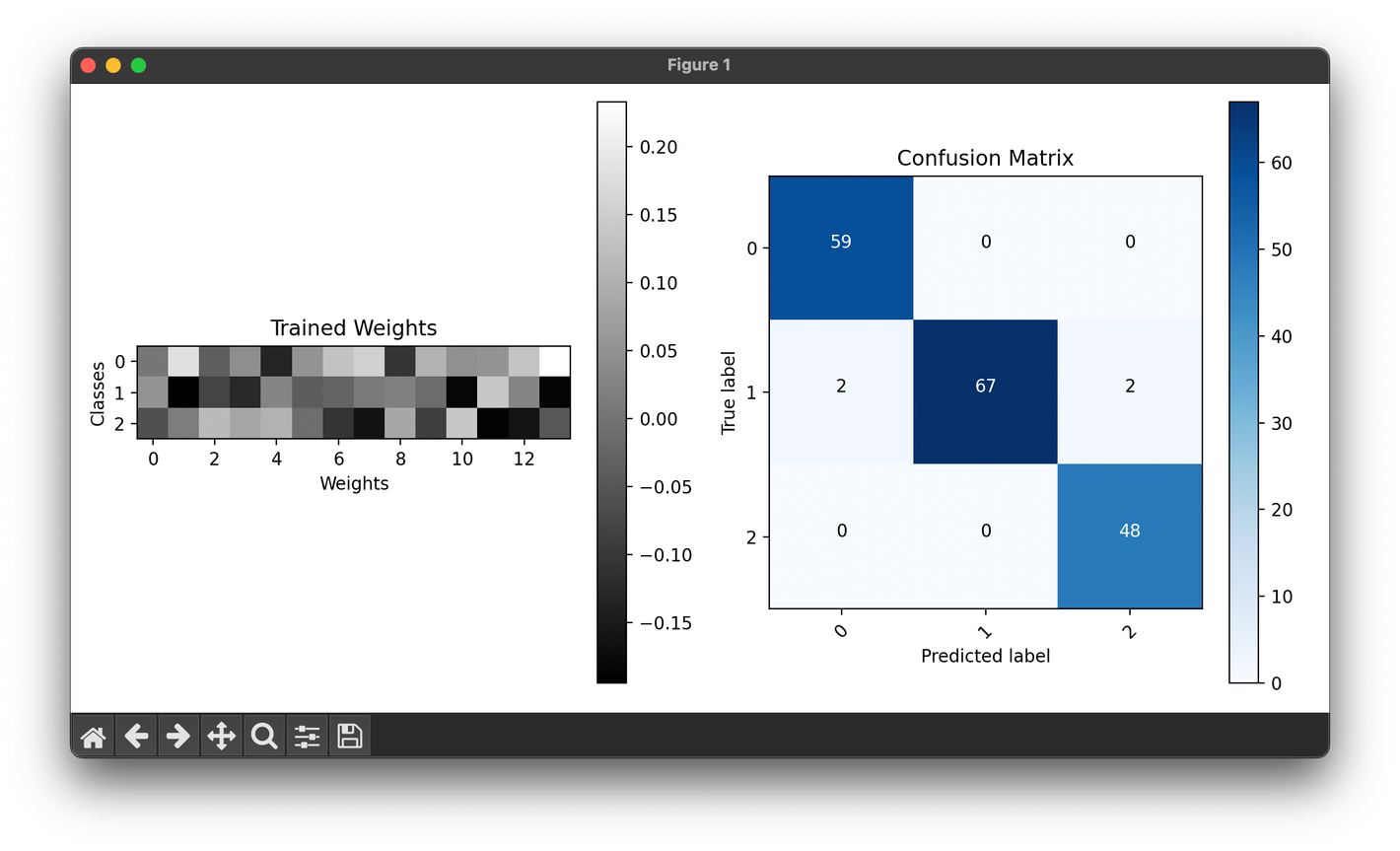

Applications

• Binary Classification: Its primary application, useful in scenarios where objects need to be categorized into two groups (e.g., spam vs. non-spam emails).
• Feature Extraction: Used as a preliminary step to reduce dimensionality before applying more sophisticated algorithms.

Strengths and Limitations

Strengths

• Simplicity: Easy to implement and understand.
• Efficiency: Requires relatively few computational resources.

Limitations

• Linear Separability: Only capable of classifying linearly separable data sets.
• Binary Outputs: Limited to binary classification tasks.

Advanced Topics

• Kernel Perceptron: Extension of the perceptron that uses kernel functions to enable it to classify non-linearly separable data.
• Multi-layer Perceptrons (MLP): Networks of perceptrons (also known as feedforward neural networks) that can model complex, non-linear relationships between inputs and outputs.

References

1. Rosenblatt, Frank. "The perceptron: A probabilistic model for information storage and organization in the brain." Psychological Review 65.6 (1958): 386.
2. Minsky, Marvin, and Seymour Papert. "Perceptrons: An introduction to computational geometry." The MIT Press, 1969.
3. Goodfellow, Ian, et al. "Deep Learning." MIT Press, 2016. 🔗