Perceptron Regression

Introduction

Perceptron regression extends the concept of the perceptron from classification to regression tasks. While a classic perceptron is designed for binary classification, predicting discrete labels, perceptron regression is adapted to predict continuous outcomes. This adaptation allows the application of the perceptron model to a wider range of problems where the goal is to predict a numeric value rather than a class label.

Mathematical Foundations

Model Representation

Similar to the perceptron for classification, the perceptron for regression also takes a vector of real-valued inputs, $\mathbf{x} = [x_1, x_2, \ldots, x_n]$, combines them with a set of weights, $\mathbf{w} = [w_1, w_2, \ldots, w_n]$, and adds a bias term $b$.

However, instead of using a step function as the activation, a linear activation function is used. This makes the output continuous rather than binary:

This equation represents the linear relationship between the input features and the target value, where $\hat{y}$ is the predicted numerical value.

Learning Algorithm

The goal of perceptron regression is to minimize the difference between the actual and predicted values. This is often achieved using a cost function such as Mean Squared Error (MSE):

Where:

• $N$ is the number of training samples,
• $y_i$ is the actual value for the $i$-th sample,
• $\hat{y}_i$ is the predicted value for the $i$-th sample.

The weights are updated to minimize the cost function, typically using gradient descent. The update rule for the weights and bias in its simplest form, using a learning rate $\eta$, looks like this:

The partial derivatives of the MSE with respect to the weights and bias give us the direction in which to update our parameters to minimize the error.

Adaptation for Regression

The key adaptation for regression tasks is the use of a continuous activation function (in this case, a linear function) and a cost function that measures the difference in continuous values. The training process involves adjusting the weights and bias to minimize this cost across all training samples.

Implementation

Parameters

• learning_rate: float, default = 0.01
  Step size for updating weights
  
• max_iter: int, default = 1000
  Maximum iteration
  
• regularization: Literal['l1', 'l2', 'elastic-net'], default = None
  Regularizing methods
  
• alpha: float, default = 0.0001
  Regularization strength
  
• l1_ratio: float, default = 0.5
  Ratio of L1 regularization in elastic-net regularization
  
• random_state: int, default = None
  Seed for random shuffling during SGD
  

Examples

from luma.neural.single import PerceptronRegressor
from luma.preprocessing.scaler import StandardScaler
from luma.preprocessing.outlier import LocalOutlierFactor
from luma.model_selection.search import RandomizedSearchCV
from luma.model_selection.split import TrainTestSplit
from luma.metric.regression import MeanSquaredError
from luma.visual.evaluation import ResidualPlot

from sklearn.datasets import load_diabetes
import matplotlib.pyplot as plt
import numpy as np

np.random.seed(42)

X, y = load_diabetes(return_X_y=True)

sc = StandardScaler()
X_std = sc.fit_transform(X)
y_std = sc.fit_transform(y)

lof = LocalOutlierFactor(n_neighbors=10, threshold=1.5)
X_fil, y_fil = lof.fit_transform(X_std, y_std)

X_train, X_test, y_train, y_test = TrainTestSplit(X_fil, y_fil, 
												  test_size=0.3).get

param_dist = {
    "learning_rate": np.logspace(-3, -1, 10),
    "alpha": np.logspace(-2, 2, 10),
    "l1_ratio": np.linspace(0, 1, 10),
    "regularization": ["l1", "l2", "elastic-net"],
}

rand = RandomizedSearchCV(
    estimator=PerceptronRegressor(max_iter=100),
    param_dist=param_dist,
    max_iter=50,
    cv=5,
    metric=MeanSquaredError,
    maximize=False,
    refit=True,
    shuffle=True,
    verbose=True,
)

rand.fit(X_train, y_train)
print(rand.best_params, rand.best_score)

X_all = np.vstack((X_train, X_test))
y_all = np.hstack((y_train, y_test))

model = rand.best_model
fig = plt.figure(figsize=(10, 5))
ax1 = fig.add_subplot(1, 2, 1)
ax2 = fig.add_subplot(1, 2, 2)

ax1.plot(range(X.shape[1] + 1), model.weights_, c="blue", marker="o", ls="--")
ax1.set_xlabel("Features")
ax1.set_ylabel("Weight")
ax1.set_title(f"Trained Weights [MSE: {model.score(X_test,y_test):.4f}]")
ax1.grid(alpha=0.2)

res = ResidualPlot(model, X_all, y_all)
res.plot(ax=ax2, show=True)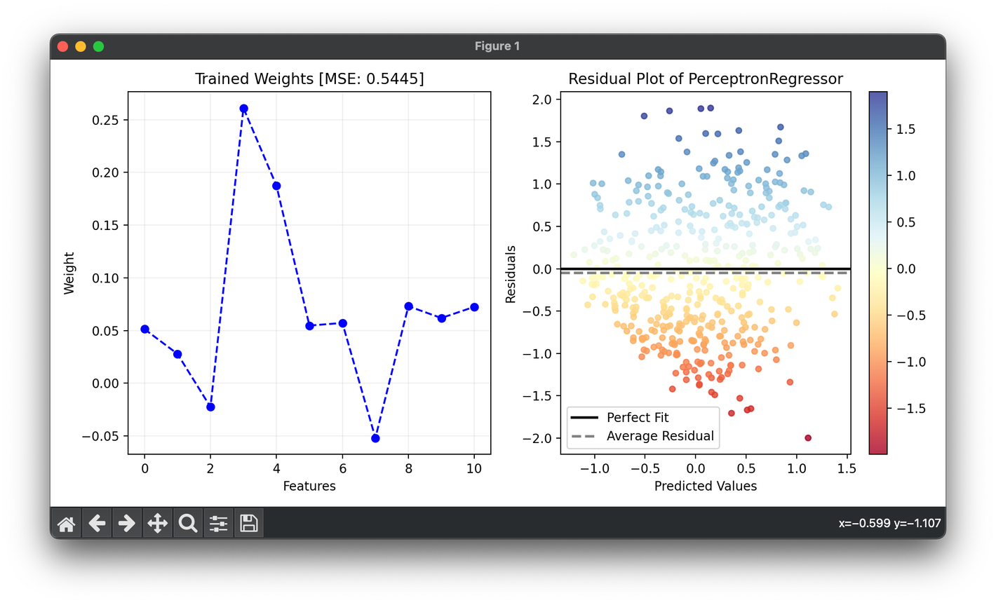

Applications

• Predicting housing prices: Given features like size, location, and number of bedrooms, predict the price of a house.
• Forecasting stock prices: Use historical data to predict future stock prices.
• Energy consumption forecasting: Predict the energy consumption of a building based on past consumption and weather data.

Strengths and Limitations

Strengths

• Simplicity and interpretability: The model is straightforward to implement and understand, making it a good baseline for regression tasks.
• Efficiency: Requires relatively few computational resources, allowing it to run quickly even on large datasets.

Limitations

• Assumption of linearity: Can only model linear relationships between inputs and outputs.
• Sensitivity to outliers: Being a linear model, it is sensitive to outliers in the data which can significantly affect the fit of the model.
• Limited complexity: Cannot capture complex patterns in data without transformation or extension to the model.

Advanced Topics

• Regularization in Perceptron Regression: Techniques like L1 (Lasso) and L2 (Ridge) regularization can be applied to perceptron regression to prevent overfitting and improve model performance on unseen data.
• Kernelized Perceptron Regression: Extending the perceptron with kernel methods to model non-linear relationships.

References

1. Bishop, Christopher M. "Pattern Recognition and Machine Learning." Springer, 2006.
2. Friedman, Jerome, et al. "The elements of statistical learning." Springer series in statistics New York, NY, USA:, 2001.
3. Hastie, Trevor, Robert Tibshirani, and Jerome Friedman. "The Elements of Statistical Learning: Data Mining, Inference, and Prediction." Springer Series in Statistics, 2009.