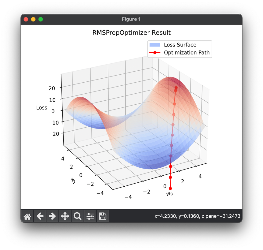
Root Mean Square Propagation (RMSProp)

Introduction

RMSProp, short for Root Mean Square Propagation, is an adaptive learning rate optimization algorithm designed to address some of the drawbacks of traditional stochastic gradient descent (SGD) methods. Introduced by Geoffrey Hinton in his Coursera course on neural networks, RMSProp modifies the learning rate for each parameter individually, making it smaller for parameters with large gradients and larger for those with small gradients. This approach helps in speeding up convergence, especially in the context of training deep neural networks with complex landscapes.

Background and Theory

The key idea behind RMSProp is to maintain a moving average of the squared gradients for each parameter and to adjust the learning rates by dividing by the square root of this average. This makes the optimizer scale down the gradient for parameters with historically large gradients and scale up the gradient for parameters with historically small gradients, thus leading to a more stable and efficient convergence.

Mathematically, RMSProp updates parameters using a moving average of the squared gradients. For a parameter $\theta$, the update rule is as follows:

1. Calculate the gradient: $g_t = \nabla_\theta L(\theta_t)$, where $L$ is the loss function.
2. Update the squared gradient moving average: $E[g^2]_t = \beta E[g^2]_{t-1} + (1 - \beta)g_t^2$, where $\beta$ is the decay rate.
3. Update the parameter: $\theta_{t+1} = \theta_t - \frac{\eta}{\sqrt{E[g^2]_t + \epsilon}} g_t$, where $\eta$ is the learning rate, and $\epsilon$ is a small constant to prevent division by zero.

Procedural Steps

1. Initialization: Initialize the parameters $\theta$ and the moving average $E[g^2]$ to zero.
2. Gradient Computation: At each step $t$, compute the gradient $g_t$ of the loss function with respect to the parameters.
3. Update Moving Average: Update the moving average of the squared gradients $E[g^2]_t$.
4. Parameter Update: Adjust the parameters $\theta$ using the updated moving average to scale the learning rate.
5. Iteration: Repeat steps 2-4 until convergence or for a fixed number of iterations.

Mathematical Formulation

The RMSProp algorithm adjusts the learning rate dynamically for each parameter. The update rule can be decomposed into two main parts:

1. Moving Average Update:

   $E[g^2]_t = \beta E[g^2]_{t-1} + (1 - \beta)g_t^2$

   This step calculates the exponential moving average of the squared gradients, where $\beta$ controls the decay rate.

2. Parameter Update:

   $\theta_{t+1} = \theta_t - \frac{\eta}{\sqrt{E[g^2]_t + \epsilon}} g_t$

   Here, $\eta$ is the global learning rate, and $\epsilon$ is a smoothing term added to the denominator to avoid division by zero.

Applications

RMSProp is widely used in training deep neural networks, particularly in situations where the optimization landscape is complex or non-convex. It has shown to be effective in various tasks, including image recognition, natural language processing, and reinforcement learning.

Strengths and Limitations

Strengths

• Adaptive Learning Rates: By adjusting the learning rate for each parameter, RMSProp can navigate the parameter space more efficiently.
• Stable Convergence: RMSProp tends to show stable convergence behavior, especially in settings with noisy or sparse gradients.

Limitations

• Hyperparameter Sensitivity: The performance of RMSProp can be sensitive to the choice of its hyperparameters, like the learning rate $\eta$ and the decay rate $\beta$.
• Lack of Theoretical Guarantee: While empirically effective, RMSProp lacks the theoretical convergence guarantees provided for some other optimization methods.

Advanced Topics

• Combination with Momentum: RMSProp can be combined with momentum to further accelerate the convergence by incorporating the moving average of gradients.
• Comparison with Other Adaptive Methods: Understanding the differences and similarities between RMSProp and other adaptive methods like AdaGrad, Adam, and AdaDelta helps in choosing the right optimizer for a specific problem.

References

1. Tieleman, Tijmen, and Geoffrey Hinton. "Lecture 6.5-rmsprop: Divide the gradient by a running average of its recent magnitude." COURSERA: Neural Networks for Machine Learning 4 (2012).