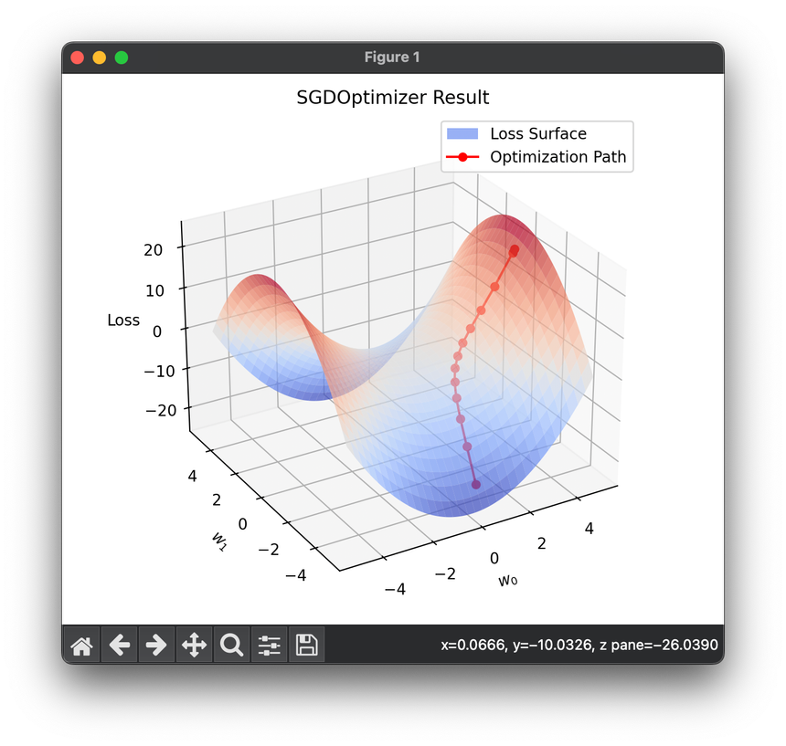
Stochastic Gradient Descent (SGD)

Introduction

Stochastic Gradient Descent (SGD) is a fundamental optimization technique used widely in machine learning and deep learning for minimizing the loss function associated with a model. The "stochastic" part of SGD refers to the fact that the gradient—the vector of partial derivatives of the loss function—is calculated with respect to a randomly selected subset of data rather than the full dataset. This approach contrasts with traditional gradient descent, which uses the entire dataset to compute the gradient at every step. SGD's popularity stems from its efficiency and effectiveness in handling large datasets and complex models.

Background and Theory

Gradient Descent (GD) forms the backbone of many optimization algorithms. It operates on the premise that if one moves in the direction opposite to the gradient of the function at a given point, it is possible to reach the local minimum of that function. Mathematically, the update rule for GD when minimizing a loss function $L(\theta)$, where $\theta$ denotes the parameters of the model, is given by:

Here, $\eta$ represents the learning rate, a hyperparameter that controls the size of the steps taken towards the minimum. $\nabla_\theta L(\theta)$ denotes the gradient of the loss function with respect to the parameters $\theta$.

SGD modifies this approach by estimating the gradient $\nabla_\theta L(\theta)$ based on a subset of the data, typically one example (mini-batch size of 1) or a small batch of examples. This estimation significantly reduces the computational burden, making it viable to train on large datasets. The update rule for SGD can be similarly expressed as:

Where $L_i(\theta)$ is the loss computed on a randomly selected subset (mini-batch) of the data.

Procedural Steps

The steps to implement SGD are as follows:

1. Initialization: Initialize the parameters $\theta$ of the model randomly or with a predefined strategy.

2. Mini-batch Selection: Randomly select a mini-batch of data points from the training set.

3. Gradient Computation: Compute the gradient of the loss function with respect to the parameters $\theta$, but only for the selected mini-batch. This gradient is an estimation of the true gradient computed on the entire dataset.

4. Parameter Update: Update the model's parameters using the estimated gradient and the learning rate $\eta$ according to the formula

   $\theta_{new} = \theta_{old} - \eta \nabla_\theta L_i(\theta)$

5. Repeat: Repeat steps 2-4 for a predefined number of iterations or until the loss converges to an acceptable value.

Mathematical Formulation

The essence of SGD lies in the gradient computation step, where the gradient $\nabla_\theta L_i(\theta)$ is an estimate of $\nabla_\theta L(\theta)$, the true gradient. For a loss function $L(\theta)$ defined over the entire dataset and a mini-batch $B$, the estimated gradient is:

where $l(x_i, y_i, \theta)$ is the loss associated with a single data point $(x_i, y_i)$, and $|B|$ is the size of the mini-batch.

Applications

SGD is universally applicable across various machine learning tasks, including but not limited to:

• Training deep neural networks for image recognition, natural language processing, and time series analysis.
• Logistic regression and other generalized linear models for classification and regression tasks.
• Support Vector Machines (SVMs) and other margin-based models.

Strengths and Limitations

Strengths

• Efficiency: SGD is highly efficient for large datasets, as it updates the model parameters without needing to compute gradients over the entire dataset.
• Online Learning: It supports online learning, where the model can be updated as new data arrives.

Limitations

• Convergence: The stochastic nature of the gradient estimation can lead to noisy updates, potentially causing the convergence to be slower or to fluctuate around the minimum.
• Hyperparameter Sensitivity: The choice of learning rate and mini-batch size significantly impacts the effectiveness and stability of the training process.

Advanced Topics

• Learning Rate Scheduling: Techniques to adjust the learning rate during training, such as step decay, exponential decay, or adaptive methods like Adam.
• Momentum and Variants: Incorporation of momentum to stabilize and accelerate convergence. Variants of SGD such as SGD with momentum, Nesterov Accelerated Gradient (NAG), and Adam incorporate adaptive learning rates or momentum to address some of SGD's limitations.

References

1. Bottou, Léon. "Large-scale machine learning with stochastic gradient descent." Proceedings of COMPSTAT'2010. Physica-Verlag HD, 2010.
2. Ruder, Sebastian. "An overview of gradient descent optimization algorithms." arXiv preprint arXiv:1609.04747 (2016).