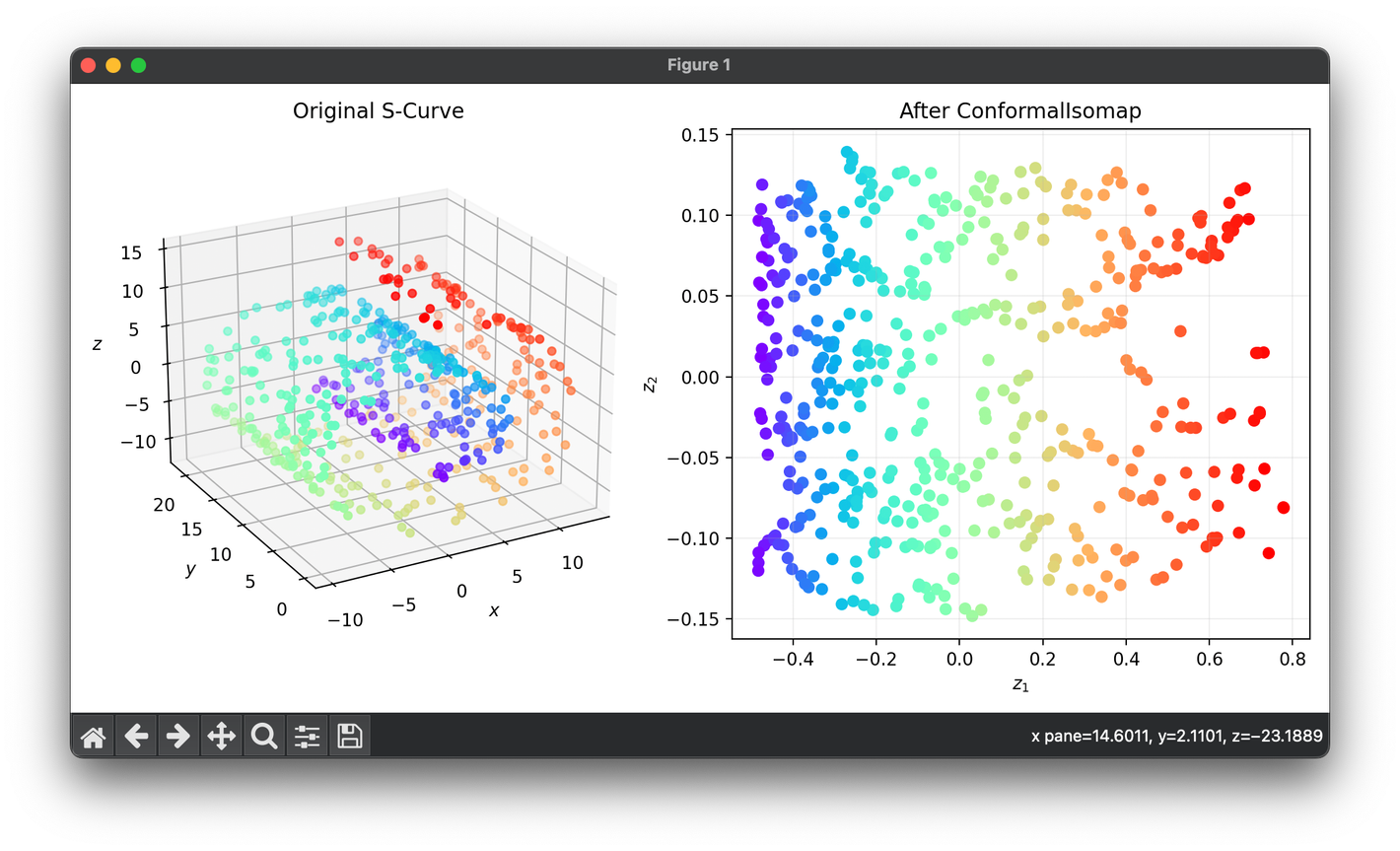
Conformal Isomap (C-Isomap)

Introduction

Conformal Isomap (C-Isomap) refines the Isometric Mapping (Isomap) technique by incorporating the principle of conformality into the dimensionality reduction process. This advanced variant is designed to not only preserve the global structure of the data but also to maintain local angles between points, making it highly suitable for applications where local geometry is critical. Through the use of Riemannian geometry, C-Isomap aims to provide a more nuanced representation of the manifold's intrinsic structure.

Background and Theory

Enhancing Isomap with Conformality

While Isomap focuses on preserving global geodesic distances, C-Isomap extends this by ensuring that the reduction process also conserves local angular relationships. This is achieved through conformal mappings, which are angle-preserving transformations within the mathematical field of Riemannian geometry.

The Concept of Conformality

Conformality in mathematics refers to transformations that preserve angles. In the context of C-Isomap, it involves adjusting the computation of distances and the dimensionality reduction process to ensure that the local structure of the data, especially the angles between points, is maintained in the reduced space.

Riemannian Geometry and Its Role

Riemannian geometry, the study of curved spaces, provides the theoretical foundation for understanding and applying conformal mappings. This framework is crucial for C-Isomap, as it allows for the precise manipulation of the manifold's local properties.

Mathematical Formulation

The core steps of C-Isomap can be mathematically expressed as follows:

1. Graph Construction with Conformal Weights:
   Construct a weighted graph $G(V, E)$, where $V$ are vertices representing the data points, and $E$ are edges weighted by Euclidean distances modified by conformal factors to reflect local geometry. This can be represented as:
   $w_{ij} = \delta(i, j) \cdot c(i, j)$
   where $w_{ij}$ is the weight of the edge between vertices $i$ and $j$, $\delta(i, j)$ is the Euclidean distance, and $c(i, j)$ is the conformal factor derived from local angular considerations.
   
2. Conformal Distance Estimation:
   Compute the conformal distances by finding the shortest paths in the weighted graph, which now incorporate both geodesic and conformal adjustments. The Floyd-Warshall or Dijkstra's algorithm may be employed here, adjusting for conformal weights.
3. Multidimensional Scaling (MDS):
   Apply MDS to the matrix of conformal distances to achieve a lower-dimensional representation that maintains both global and local properties. The goal is to minimize the stress function:
   $\text{Stress}(D, D') = \sqrt{\sum_{i < j} (\delta'(i, j) - d_{ij})^2}$
   where $D$ is the matrix of conformal distances in the high-dimensional space, $D'$ is the matrix of distances in the reduced space, $\delta'(i, j)$ represents the distances in the reduced space, and $d_{ij}$ are the original conformal distances.
   

Procedural Steps

1. Data Preprocessing: Standardize the dataset to ensure equal weighting of features.
2. Graph Construction: Create a neighborhood graph, adjusting edge weights for conformality based on the local angles and Riemannian metrics.
3. Distance Calculation: Determine the shortest paths that reflect conformal distances, taking into account both the manifold's curvature and local angle preservation.
4. Dimensionality Reduction: Employ MDS on the conformal distance matrix to project the data into a lower-dimensional space, striving to keep intact the data's global structure and local angular relationships.

Implementation

Parameters

• n_components: int
  Dimensionality of low-space
  
• epsilon: float, default = 5.0
  Boundary radius of the neighbor hypersphere
  
• algorithm: Literal['dijkstra', 'floyd'], default = ‘dijkstra’
  Shortest path finding algorithm, i.e. Dijkstra’s algorithm($O(n^2)$), Floyd-Warshall algorithm($O(n^3)$)
  

Examples

from luma.reduction.manifold import ConformalIsomap

from sklearn.datasets import make_swiss_roll
import matplotlib.pyplot as plt

X, y = make_swiss_roll(n_samples=500, noise=0.2)

model = ConformalIsomap(n_components=2, epsilon=5, algorithm='dijkstra')
Z = model.fit_transform(X)

fig = plt.figure(figsize=(10, 5))
ax1 = fig.add_subplot(1, 2, 1, projection="3d")
ax2 = fig.add_subplot(1, 2, 2)

ax1.scatter(X[:, 0], X[:, 1], X[:, 2], c=y, cmap="rainbow")
ax1.set_xlabel(r"$x$")
ax1.set_ylabel(r"$y$")
ax1.set_zlabel(r"$z$")
ax1.set_title("Original S-Curve")

ax2.scatter(Z[:, 0], Z[:, 1], c=y, cmap="rainbow")
ax2.set_xlabel(r"$z_1$")
ax2.set_ylabel(r"$z_2$")
ax2.set_title(f"After {type(model).__name__}")
ax2.grid(alpha=0.2)

plt.tight_layout()
plt.show()

Applications

C-Isomap's ability to preserve local angles makes it particularly effective in:

• Medical Imaging Analysis: Where local structural details are critical for diagnosing conditions.
• Computer Graphics and 3D Modeling: For accurate texture mapping and geometric transformations.
• Robotics and Navigation: Where understanding the local spatial relationships is essential for path planning and environmental understanding.

Strengths and Limitations

Strengths

• Preservation of Local Geometry: Ensures that small-scale structures are maintained, crucial for datasets where local details are significant.
• Comprehensive Dimensionality Reduction: Offers a more detailed representation by preserving both global and local data structures.

Limitations

• Computational Complexity: The inclusion of conformal weights and the calculation of Riemannian metrics increases the computational demands.
• Sensitivity to Parameters: The choice of neighbors and the calculation of conformal factors can significantly influence the outcome.
• Potential for Overfitting: There's a risk of overemphasizing local features, which may distort the global structure's representation.

Advanced Topics

• Efficiency Improvements: Research into algorithmic optimizations to handle larger datasets with reduced computational overhead.
• Hybrid Manifold Learning Approaches: Combining C-Isomap with other dimensionality reduction techniques to leverage their strengths.
• Deep Learning Integration: Investigating how C-Isomap can be embedded into neural network architectures for enhanced feature extraction and representation learning.