Laplacian Eigenmap

Introduction

Laplacian Eigenmap is a dimensionality reduction technique used in machine learning and data science to project high-dimensional data into a lower-dimensional space, preserving the local structure of the data. Unlike other linear techniques such as Principal Component Analysis (PCA), Laplacian Eigenmap is a non-linear method that focuses on maintaining local distances between data points, which makes it particularly useful for data that lies on a manifold.

The technique is rooted in the field of spectral graph theory and is designed to uncover the intrinsic geometry of data represented as a graph. By constructing a neighborhood graph from the data points, Laplacian Eigenmap uses the graph Laplacian's eigenvalues and eigenvectors to find a low-dimensional representation that best preserves the graph's local properties.

Background and Theory

Mathematical Foundations

To understand Laplacian Eigenmaps, it's essential to grasp some underlying mathematical concepts, primarily those related to graph theory and spectral analysis.

Graph Theory Basics

A graph $G = (V, E)$ consists of a set of vertices $V$ and a set of edges $E$ connecting these vertices. In the context of Laplacian Eigenmaps, vertices represent data points, and edges represent the connections between them, typically based on some notion of similarity or proximity.

Graph Laplacian

The graph Laplacian is a matrix representation that characterizes the difference between a vertex and its neighbors. It's defined as $L = D - W$, where:

• $L$ is the Laplacian matrix.
• $W$ is the weight matrix, with $W_{ij}$ representing the weight of the edge between vertices $i$ and $j$. Weights are often assigned based on the Euclidean distance between points, with closer points assigned higher weights.
• $D$ is the degree matrix, a diagonal matrix where each diagonal element $D_{ii}$ is the sum of the weights of all edges connected to vertex $i$.

The graph Laplacian plays a central role in Laplacian Eigenmaps, as it captures the essential structure of the data.

The Laplacian Eigenmap Algorithm

The objective of the Laplacian Eigenmap algorithm is to find a low-dimensional representation of the data that preserves local distances. This is achieved through the eigenvalue decomposition of the Laplacian matrix $L$. Specifically, the algorithm involves the following steps:

1. Construct the neighborhood graph: Create a graph where each point is connected to its $k$ nearest neighbors or to all neighbors within a certain radius $\epsilon$.
2. Choose the weights: Assign weights to the edges, typically using the heat kernel $W_{ij} = \exp(-{\|x_i - x_j\|^2}/t)$ for an edge between $x_i$ and $x_j$, where $t$ is a parameter controlling the width of the neighborhood.
3. Compute the Laplacian matrix: Calculate $L = D - W$.
4. Eigenvalue decomposition: Solve the generalized eigenvalue problem $Lv = \lambda Dv$ for the smallest eigenvalues and their corresponding eigenvectors.
5. Construct the embedding: Select the eigenvectors corresponding to the smallest non-zero eigenvalues (excluding the trivial solution) to form the new coordinates in the low-dimensional space.

Implementation

Parameters

• n_components: int
  Dimensionality of the lower-dimensional space
  
• sigma: float, default = 1.0
  Width parameter for Gaussian kernel in affinity calculation
  

Examples

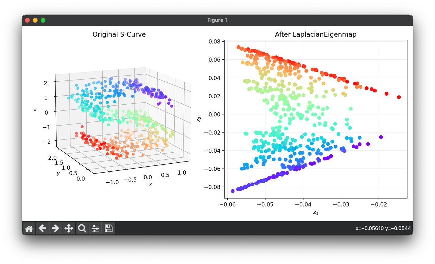
from luma.reduction.manifold import LaplacianEigenmap

from sklearn.datasets import make_s_curve
import matplotlib.pyplot as plt

X, y = make_s_curve(n_samples=500, noise=0.1)

model = LaplacianEigenmap(n_components=2, sigma=0.3)
Z = model.fit_transform(X)

fig = plt.figure(figsize=(10, 5))
ax1 = fig.add_subplot(1, 2, 1, projection="3d")
ax2 = fig.add_subplot(1, 2, 2)

ax1.scatter(X[:, 0], X[:, 1], X[:, 2], c=y, cmap="rainbow")
ax1.set_xlabel(r"$x$")
ax1.set_ylabel(r"$y$")
ax1.set_zlabel(r"$z$")
ax1.set_title("Original S-Curve")

ax2.scatter(Z[:, 0], Z[:, 1], c=y, cmap="rainbow")
ax2.set_xlabel(r"$z_1$")
ax2.set_ylabel(r"$z_2$")
ax2.set_title(f"After {type(model).__name__}")
ax2.grid(alpha=0.2)

plt.tight_layout()
plt.show()

Applications

• Image and video processing: For tasks like image segmentation and motion capture data analysis, where preserving the local pixel or frame relationships is crucial.
• Natural Language Processing (NLP): For word embeddings where similar words are desired to be close in the embedding space.
• Bioinformatics: In gene expression data analysis, for identifying clusters of genes with similar expression patterns.

Strengths and Limitations

Strengths

• Preserves local structure: Ideal for data with inherent geometric or manifold structures.
• Flexibility: Works well with various definitions of neighborhood and distance metrics.
• Non-linear: Capable of uncovering non-linear structures that linear methods like PCA cannot.

Limitations

• Scale sensitivity: The choice of parameters such as the neighborhood size can significantly affect the results.
• Computational complexity: The eigenvalue decomposition can be computationally intensive for large datasets.
• Out-of-sample data: Laplacian Eigenmap does not naturally extend to new, unseen data points, requiring additional methods for out-of-sample extensions.

Advanced Topics

Out-of-Sample Extensions

Extending Laplacian Eigenmap to new data points requires techniques such as the Nyström method, which approximates the eigenfunctions of the Laplacian matrix for out-of-sample data based on a subset of the original data.

Kernelized Laplacian Eigenmaps

Kernel methods can be integrated with Laplacian Eigenmaps to capture more complex data structures, leading to a more flexible approach that can handle a broader range of datasets.

References

1. Belkin, Mikhail, and Partha Niyogi. "Laplacian Eigenmaps for Dimensionality Reduction and Data Representation." Neural Computation, vol. 15, no. 6, 2003, pp. 1373-1396.
2. Von Luxburg, Ulrike. "A tutorial on spectral clustering." Statistics and computing 17.4 (2007): 395-416.