Landmark Multidimensional Scaling (Landmark MDS)

Introduction

Landmark Multidimensional Scaling (Landmark MDS) is an advanced variation of the classical Multidimensional Scaling (MDS) technique, which is aimed at dimensionality reduction and visualization of high-dimensional data. The primary goal of Landmark MDS is to map high-dimensional data points into a lower-dimensional space while preserving the pairwise distances between points as much as possible. This method is particularly useful for visualizing similarities or dissimilarities within large datasets. Landmark MDS distinguishes itself by selecting a subset of the data points as "landmarks" and using these to guide the dimensionality reduction process, making it significantly more efficient and scalable compared to traditional MDS methods.

Background and Theory

Multidimensional Scaling (MDS)

At its core, MDS is a set of data analysis techniques that visualize the level of similarity of individual cases of a dataset. Classical MDS focuses on distance matrices and attempts to find a low-dimensional representation of the data that preserves these distances. The primary objective can be mathematically formulated as minimizing the stress function, which quantifies the difference between the distances in the high-dimensional and the low-dimensional spaces.

Landmark MDS

Landmark MDS improves upon classical MDS by introducing the concept of landmarks. These are a strategically selected subset of the data points that serve as a reference or "basis" in the dimensionality reduction process. The selection of landmarks is crucial and can be done through various strategies, such as random selection, farthest point sampling, or based on data density.

Mathematical Foundations

Given a high-dimensional dataset $X = \{\mathbf{x}_1, \mathbf{x}_2, \ldots, \mathbf{x}_n\}$ where each $\mathbf{x}_i \in \mathbb{R}^d$, the goal is to find a low-dimensional representation $Y = \{\mathbf{y}_1, \mathbf{y}_2, \ldots, \mathbf{y}_n\}$ where each $\mathbf{y}_i \in \mathbb{R}^k$ and $k < d$, such that the pairwise distances $D(X)$ in the high-dimensional space are preserved as much as possible in $D(Y)$, the pairwise distances in the low-dimensional space.

The stress function, commonly used to measure the fidelity of the low-dimensional representation, is defined as:

where $d_{ij}$ is the distance between points $\mathbf{x}_i$ and $\mathbf{x}_j$ in the high-dimensional space, and $\| \mathbf{y}_i - \mathbf{y}_j \|$ is the Euclidean distance between points $\mathbf{y}_i$ and $\mathbf{y}_j$ in the low-dimensional representation.

For Landmark MDS, let $L \subset X$ be the set of landmarks. The distance matrix $D(L, X)$, representing distances between landmarks and all other points, is computed. The optimization process then focuses on preserving these distances in the low-dimensional space, which can be achieved more efficiently due to the reduced size of $L$.

Procedural Steps

1. Landmark Selection: Identify a subset of the data points as landmarks. This can be done randomly or through more sophisticated methods like farthest point sampling.
2. Distance Matrix Calculation: Calculate the distance matrix $D(L, X)$, which includes distances between landmarks and all other points.
3. Optimization: Apply optimization techniques to find a low-dimensional representation $Y$ that minimizes the stress function, focusing on preserving the distances $D(L, X)$.
4. Dimensionality Reduction for Non-landmarks: Once the landmarks are positioned in the low-dimensional space, the positions of the non-landmark points are determined based on their distances to the landmarks.

Implementation

Parameters

• n_components: int, default = None
  Dimensionality of low-space
  
• n_landmarks: int, default = 10
  Number of landmarks
  
• method: Literal['random', 'kmeans, 'kmeans++', 'kmedians'], default = ‘random’
  Algorithm for landmark initialization
  

Examples

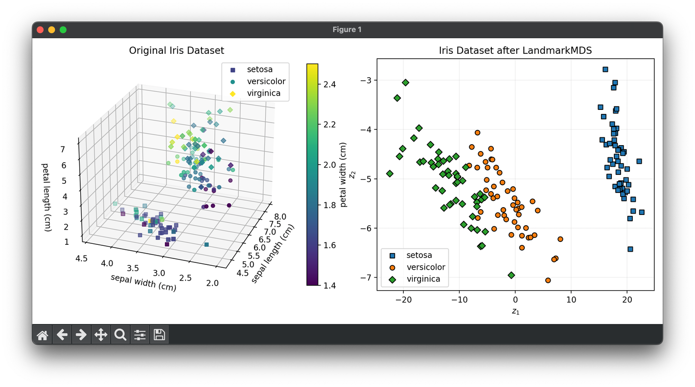
Test on the wine dataset:

from luma.reduction.manifold import LandmarkMDS

from sklearn.datasets import load_iris

import matplotlib.pyplot as plt
import numpy as np

iris_df = load_iris()
X = iris_df.data
y = iris_df.target

model = LandmarkMDS(n_components=2, n_landmarks=10, method="kmeans++")
X_trans = model.fit_transform(X)

fig = plt.figure(figsize=(11, 5))
ax1 = fig.add_subplot(1, 2, 1, projection="3d")
ax2 = fig.add_subplot(1, 2, 2)

for cl, m in zip(np.unique(y), ["s", "o", "D"]):
    X_cl = X[y == cl]
    sc = ax1.scatter(
        X_cl[:, 0],
        X_cl[:, 1],
        X_cl[:, 2],
        c=X_cl[:, 3],
        marker=m,
        label=iris_df.target_names[cl],
    )

ax1.set_xlabel(iris_df.feature_names[0])
ax1.set_ylabel(iris_df.feature_names[1])
ax1.set_zlabel(iris_df.feature_names[2])
ax1.set_title("Original Iris Dataset")
ax1.legend()

cbar = ax1.figure.colorbar(sc, fraction=0.04)
cbar.set_label(iris_df.feature_names[3])

for cl, m in zip(np.unique(y), ["s", "o", "D"]):
    X_tr_cl = X_trans[y == cl]
    ax2.scatter(
        X_tr_cl[:, 0],
        X_tr_cl[:, 1],
        marker=m,
        edgecolors="black",
        label=iris_df.target_names[cl],
    )

ax2.set_xlabel(r"$z_1$")
ax2.set_ylabel(r"$z_2$")
ax2.set_title(f"Iris Dataset after {type(model).__name__}")
ax2.legend()
ax2.grid(alpha=0.2)

plt.tight_layout()
plt.show()

Applications

Landmark MDS is particularly useful in fields where high-dimensional data visualization is essential, such as bioinformatics, social network analysis, and pattern recognition. Its efficiency and scalability make it suitable for datasets that are too large for classical MDS methods.

Strengths and Limitations

Strengths

• Efficiency: By reducing the optimization problem to a subset of landmarks, Landmark MDS can handle larger datasets more efficiently than classical MDS.
• Scalability: It scales better with the size of the dataset, making it practical for high-dimensional data analysis.

Limitations

• Dependency on Landmark Selection: The quality of the low-dimensional representation significantly depends on the selection of landmarks.
• Approximation: Since it's an approximation method, it may not preserve distances as accurately as classical MDS in some cases.

Advanced Topics

• Landmark Selection Strategies: Investigating different strategies for selecting landmarks can significantly impact the performance and outcome of Landmark MDS.
• Integration with Machine Learning Models: Landmark MDS can be combined with machine learning models for tasks such as dimensionality reduction before clustering or classification.

References

1. Cox, Trevor F., and Michael A. A. Cox. "Multidimensional Scaling." Chapman and Hall/CRC, 2001.
2. De Silva, Vin, and Joshua B. Tenenbaum. "Global versus local methods in nonlinear dimensionality reduction." Advances in neural information processing systems, 2002.
3. Yang, Zhen, et al. "Distance metric learning: A comprehensive survey." Michigan State Universiy, 2006.