Metric Multidimensional Scaling (Metric MDS)

Introduction

Metric Multidimensional Scaling (Metric MDS) is a form of Multidimensional Scaling (MDS) that focuses on preserving the metric distances between points in a high-dimensional space when mapping them to a lower-dimensional space. Unlike Nonmetric MDS, which aims to preserve the rank order of distances, Metric MDS attempts to preserve the actual distances as closely as possible. This technique is particularly useful in applications where the precise distances between data points are crucial for analysis, such as in certain psychological, biological, and physical sciences research.

Background and Theory

Metric MDS is based on classical scaling theory, which assumes that the distance matrix used as input is derived from points in a Euclidean space. The primary goal is to find a configuration of points in a lower-dimensional space that minimizes the difference between the distances in this space and the original distances in the high-dimensional space.

Mathematical Foundations

Given a set of $n$ items with an $n \times n$ distance matrix $\mathbf{D}$, where $d_{ij}$ represents the distance between items $i$ and $j$, Metric MDS seeks to find a set of $n$ points in a $p$-dimensional space ($p < n$) such that the Euclidean distances between these points, denoted as $\hat{d}_{ij}$, closely match the original distances $d_{ij}$. The objective function, often referred to as the stress or strain, is minimized during the process:

This optimization problem is typically solved using iterative methods, such as gradient descent or majorization techniques, to find the best lower-dimensional representation of the data.

Procedural Steps

1. Input Data: Begin with an $n \times n$ distance matrix $\mathbf{D}$, representing the distances between each pair of items.
2. Double Centering: Perform double centering on $\mathbf{D}$ to convert distance measurements into a form suitable for eigenvalue decomposition. This involves calculating a matrix $\mathbf{B}$ where $\mathbf{B} = -\frac{1}{2} \mathbf{J} \mathbf{D}^2 \mathbf{J}$, and $\mathbf{J}$ is a centering matrix.
3. Eigenvalue Decomposition: Compute the eigenvalue decomposition of $\mathbf{B}$ to obtain the eigenvalues and eigenvectors. The eigenvectors corresponding to the largest eigenvalues will form the basis of the lower-dimensional space.
4. Configuration Formation: Select the $p$ largest eigenvalues and their corresponding eigenvectors to construct the coordinates of the points in the lower-dimensional space.
5. Dimension Selection: Decide the number of dimensions $p$ based on the eigenvalues or through criteria such as the scree plot or cumulative explained variance.
6. Output: The final configuration of points in the selected lower-dimensional space, aiming to preserve the original distances as closely as possible.

Implementation

Parameters

• n_components: int, default = None
  Dimensionality of low-space
  
• p: float int, default = None
  Power factor for Minkowski distance metric
  
• metric: Literal, default = ‘euclidean’
  Distance metric
  

Examples

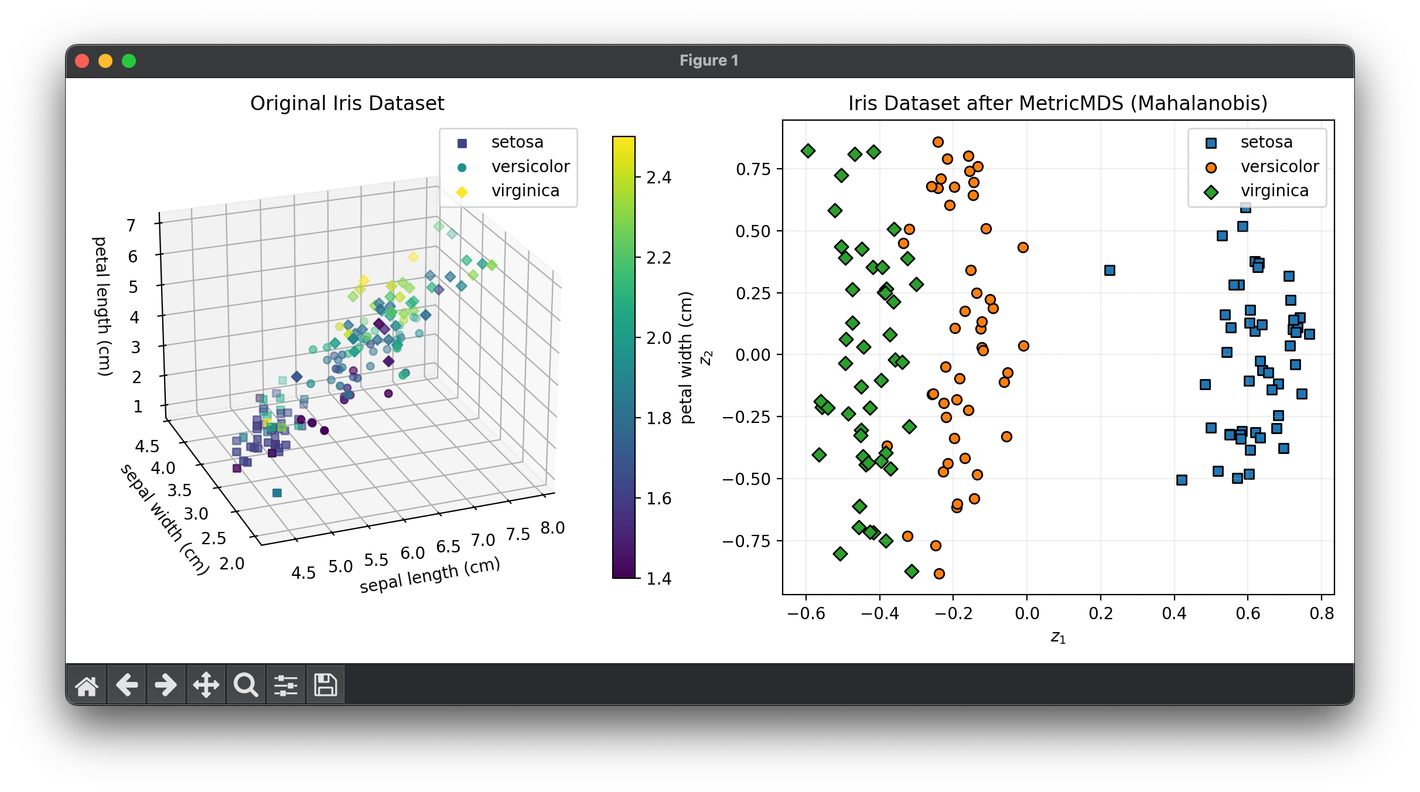
from luma.reduction.manifold import MetricMDS

from sklearn.datasets import load_iris

import matplotlib.pyplot as plt
import numpy as np

iris_df = load_iris()
X = iris_df.data
y = iris_df.target

model = MetricMDS(n_components=2, metric='mahalanobis')
X_trans = model.fit_transform(X)

fig = plt.figure(figsize=(11, 5))
ax1 = fig.add_subplot(1, 2, 1, projection="3d")
ax2 = fig.add_subplot(1, 2, 2)

for cl, m in zip(np.unique(y), ["s", "o", "D"]):
    X_cl = X[y == cl]
    sc = ax1.scatter(
        X_cl[:, 0],
        X_cl[:, 1],
        X_cl[:, 2],
        c=X_cl[:, 3],
        marker=m,
        label=iris_df.target_names[cl],
    )

ax1.set_xlabel(iris_df.feature_names[0])
ax1.set_ylabel(iris_df.feature_names[1])
ax1.set_zlabel(iris_df.feature_names[2])
ax1.set_title("Original Iris Dataset")
ax1.legend()

cbar = ax1.figure.colorbar(sc, fraction=0.04)
cbar.set_label(iris_df.feature_names[3])

for cl, m in zip(np.unique(y), ["s", "o", "D"]):
    X_tr_cl = X_trans[y == cl]
    ax2.scatter(
        X_tr_cl[:, 0],
        X_tr_cl[:, 1],
        marker=m,
        edgecolors="black",
        label=iris_df.target_names[cl],
    )

ax2.set_xlabel(r"$z_1$")
ax2.set_ylabel(r"$z_2$")
ax2.set_title(
    f"Iris Dataset after {type(model).__name__} (Mahalanobis)"
)
ax2.legend()
ax2.grid(alpha=0.2)

plt.tight_layout()
plt.show()

Applications

• Psychological Scaling: In constructing perceptual maps of consumer preferences or attitudes.
• Biological Sciences: For visualizing genetic distance or similarities among species or individuals.
• Physical Sciences: In analyzing spatial structures and relationships in physics and chemistry datasets.

Strengths and Limitations

Strengths

• Accuracy in Distance Preservation: Metric MDS is effective in preserving the actual metric distances, making it suitable for applications where these distances carry significant meaning.
• Quantitative Analysis: Enables quantitative analysis of distances and dimensional representations.

Limitations

• Dependence on Euclidean Assumption: Assumes that the input distances are Euclidean, which may not always be the case.
• Sensitivity to Outliers: Metric MDS can be sensitive to outliers or errors in the distance matrix, potentially skewing the results.
• Computational Complexity: The eigenvalue decomposition step can be computationally intensive for large datasets.

Advanced Topics

• Comparative Analysis with Nonmetric MDS: Exploring differences in applications and outcomes between metric and nonmetric MDS.
• Hybrid Approaches: Combining Metric MDS with other dimensionality reduction techniques to overcome limitations or enhance visualization.
• Robust MDS: Developing methods to make Metric MDS more resilient to outliers and non-Euclidean distances.

Reference

1. Cox, Trevor F., and Michael A. A. Cox. Multidimensional Scaling. Chapman and Hall/CRC, 2001.
2. Borg, Ingwer, and Patrick J. F. Groenen. Modern Multidimensional Scaling: Theory and Applications. Springer Science & Business Media, 2005.
3. Kruskal, Joseph B., and Myron Wish. Multidimensional Scaling. Sage Publications, 1978.