Principal Component Analysis (PCA)

Introduction

Principal Component Analysis (PCA) is a statistical procedure that uses an orthogonal transformation to convert a set of observations of possibly correlated variables into a set of values of linearly uncorrelated variables called principal components. The number of principal components is less than or equal to the number of original variables. This transformation is defined in such a way that the first principal component has the largest possible variance (that is, accounts for as much of the variability in the data as possible), and each succeeding component, in turn, has the highest variance possible under the constraint that it is orthogonal to the preceding components. The resulting vectors (principal components) are an uncorrelated orthogonal basis set. PCA is sensitive to the relative scaling of the original variables.

Background and Theory

PCA is founded on the method of eigenvalue decomposition of a data covariance (or correlation) matrix or singular value decomposition (SVD) of a data matrix, usually after mean centering (and normalizing or using Z-scores) the data matrix for each attribute. The PCA transformation can be considered as identifying the "axes" that maximize the variance of the data.

Mathematical Foundations

Given a matrix $X$ of dimensions $n \times p$ representing $n$ observations of $p$ variables, PCA aims to find a transformation matrix $P$ that transforms $X$ into a new matrix $Y$ of dimensions $n \times p$ in which each row is an observation described in the principal components space.

1. Standardization: Often, the first step is to standardize $X$, resulting in a matrix $\hat{X}$, where each column has zero mean and unit variance.

   $\hat{x}_{ij} = \frac{x_{ij} - \mu_j}{\sigma_j}$

2. Covariance Matrix Computation: Compute the covariance matrix $\Sigma$ from $\hat{X}$.

   $\Sigma = \frac{1}{n-1} \hat{X}^T \hat{X}$

3. Eigen Decomposition: Solve for the eigenvalues $\lambda_i$ and eigenvectors $v_i$ of $\Sigma$.

   $\Sigma v_i = \lambda_i v_i$

4. Select Principal Components: Sort the eigenvectors by decreasing eigenvalues and choose the first $k$ eigenvectors. This forms the transformation matrix $P$.

5. Transformation: Transform $\hat{X}$ using $P$ to obtain the principal components $Y$.

   $Y = \hat{X}P$

Dimensionality Reduction

By selecting a subset $k < p$ of the principal components, PCA achieves dimensionality reduction while preserving as much of the data's variation as possible.

Procedural Steps

1. Data Preparation: Center and, if necessary, standardize the variables.
2. Covariance Matrix Analysis: Compute the covariance or correlation matrix.
3. Eigenvalue Decomposition: Perform eigenvalue decomposition on the covariance matrix.
4. Principal Component Selection: Decide the number of principal components to retain.
5. Data Projection: Project the data onto the space spanned by the selected principal components.

Implmentation

Parameters

• n_components: int
  Number of principal components
  

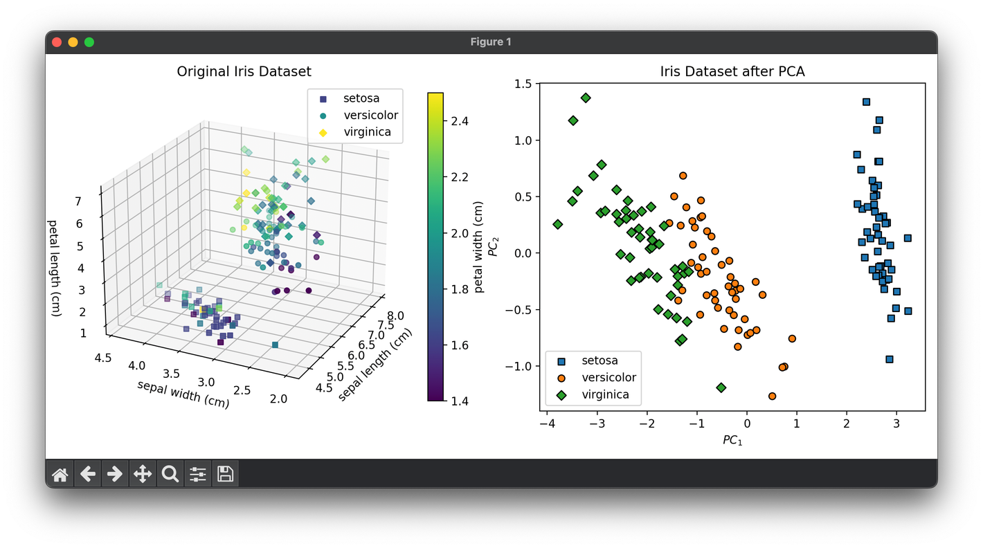
Examples

from luma.reduction.linear import PCA

from sklearn.datasets import load_iris

import matplotlib.pyplot as plt
import numpy as np

iris_df = load_iris()
X = iris_df.data
y = iris_df.target

model = PCA(n_components=2)
X_trans = model.fit_transform(X)

fig = plt.figure(figsize=(11, 5))
ax1 = fig.add_subplot(1, 2, 1, projection='3d')
ax2 = fig.add_subplot(1, 2, 2)

for cl, m in zip(np.unique(y), ['s', 'o', 'D']):
    X_cl = X[y == cl]
    sc = ax1.scatter(X_cl[:, 0], X_cl[:, 1], X_cl[:, 2], 
                     c=X_cl[:, 3], 
                     marker=m, 
                     label=iris_df.target_names[cl])

ax1.set_xlabel(iris_df.feature_names[0])
ax1.set_ylabel(iris_df.feature_names[1])
ax1.set_zlabel(iris_df.feature_names[2])
ax1.set_title('Original Iris Dataset')
ax1.legend()

cbar = ax1.figure.colorbar(sc, fraction=0.04)
cbar.set_label(iris_df.feature_names[3])

for cl, m in zip(np.unique(y), ['s', 'o', 'D']):
    X_tr_cl = X_trans[y == cl]
    ax2.scatter(X_tr_cl[:, 0], X_tr_cl[:, 1],
                marker=m, 
                edgecolors='black', 
                label=iris_df.target_names[cl])

ax2.set_xlabel(r'$PC_1$')
ax2.set_ylabel(r'$PC_2$')
ax2.set_title(f'Iris Dataset after {type(model).__name__}')
ax2.legend()

plt.tight_layout()
plt.show()

Applications

• Data Visualization: Reducing the dimensionality for visualization purposes.
• Noise Reduction: Eliminating noise by selecting a subset of principal components.
• Feature Extraction and Data Compression: Reducing the number of variables while retaining the essential information.
• Preprocessing for Machine Learning: Improving the performance of machine learning algorithms by reducing the dimensionality of the input data.

Strengths and Limitations

Strengths

• Versatility: Applicable to almost any data set, providing insights into the structure of the data.
• Data Compression: Efficiently reduces dimensionality, often with minimal loss of information.
• Simplicity: The algorithm is straightforward to implement and interpret.

Limitations

• Linearity: Assumes linear relationships among variables.
• Sensitivity to Scaling: Results depend on the scaling of the variables.
• Variance-based Selection: Principal components are selected based on variance, which might not always be the most relevant criterion.

Advanced Topics

• Kernel PCA: Extension of PCA for nonlinear dimensionality reduction through the use of kernels.
• Sparse PCA: Variation of PCA where some components are constrained to be zero for interpretability and efficiency.
• Incremental PCA: Algorithms designed for large datasets, allowing for PCA to be applied in a piecewise manner.

References

1. Jolliffe, I. T. "Principal Component Analysis." Springer Series in Statistics. Springer, New York, NY, 2002.
2. Abdi, H., and Williams, L.J. "Principal component analysis." Wiley Interdisciplinary Reviews: Computational Statistics, 2(4):433-459, 2010.
3. Pearson, K. "On Lines and Planes of Closest Fit to Systems of Points in Space." Philosophical Magazine, 2(11):559–572, 1901.
4. Hotelling, H. "Analysis of a complex of statistical variables into principal components." Journal of Educational Psychology, 24:417–441, 1933.