Sequential Backward Selection (SBS)

Sequential Backward Selection (SBS) is a feature selection technique used in machine learning to reduce the dimensionality of the data by sequentially removing features until the desired number of features is reached. This method is particularly useful in scenarios where the presence of irrelevant, redundant, or noise features may degrade the performance of a model. SBS iteratively evaluates the contribution of each feature to the model's performance and removes the least significant feature at each step.

Introduction

In the realm of machine learning and pattern recognition, the curse of dimensionality is a common problem. High-dimensional datasets can significantly impact the computational complexity and performance of machine learning algorithms. Feature selection methods, like Sequential Backward Selection, aim to mitigate these issues by selecting a subset of relevant features for model building. SBS specifically focuses on eliminating features with minimal loss to performance, thereby simplifying the model, reducing overfitting, and enhancing generalization capabilities.

Background and Theory

Sequential Backward Selection operates on the premise that eliminating certain features can lead to a simpler model without significantly compromising accuracy. The process involves the following steps:

1. Initialization: Start with the full set of $n$ features.
2. Evaluation: Compute the criterion function (e.g., model accuracy) for the subset of features.
3. Elimination: Identify and remove the feature whose exclusion leads to the least decrease or the most increase in the performance metric.
4. Termination: Repeat steps 2 and 3 until the desired number of features is achieved or further removal of features results in a significant decrease in performance.

The performance criterion function is pivotal in SBS. It evaluates the merit of a feature subset by measuring the performance of a model trained on this subset. Common criteria include classification accuracy, error rate, or any other relevant metric depending on the problem and model used.

Mathematical Formulation

Given a dataset $D$ with $n$ features, let $F = \{f_1, f_2, \ldots, f_n\}$ be the set of all features. The goal is to find a subset $F^* \subseteq F$ such that the performance metric $P(F')$ is maximized, and $|F^*|$ equals the desired number of features. The performance metric $P$ can be defined as:

where $\text{Model}_{F'}$ is the machine learning model trained on the subset of features $F'$.

At each iteration $i$, the feature to be removed, $f_{\text{remove}}$, is determined as:

where $F_{i-1}$ is the feature set from the previous iteration and $\Delta P$ represents the change in performance metric upon the removal of feature $f$.

Implementation

Parameters

• estimator: Estimator
  An estimator to fit and evaluate
  
• n_features: float int, default = 1
  Number of features to select (0~1 value for proportion)
  
• metric: Evaluator
  Scoring metric for selecting features
  
• test_size: float, default = 0.2
  Proportional size of the validation set
  
• cv: int, default = 5
  K-fold size for cross validation (0 to disable CV)
  
• shuffle: bool, default = True
  Whether to shuffle the dataset
  
• stratify: bool, default = False
  Whether to perform stratified split
  
• fold_type: FoldType, default = KFold
  Fold type
  
• random_state: float
  Seed for splitting the data
  

Examples

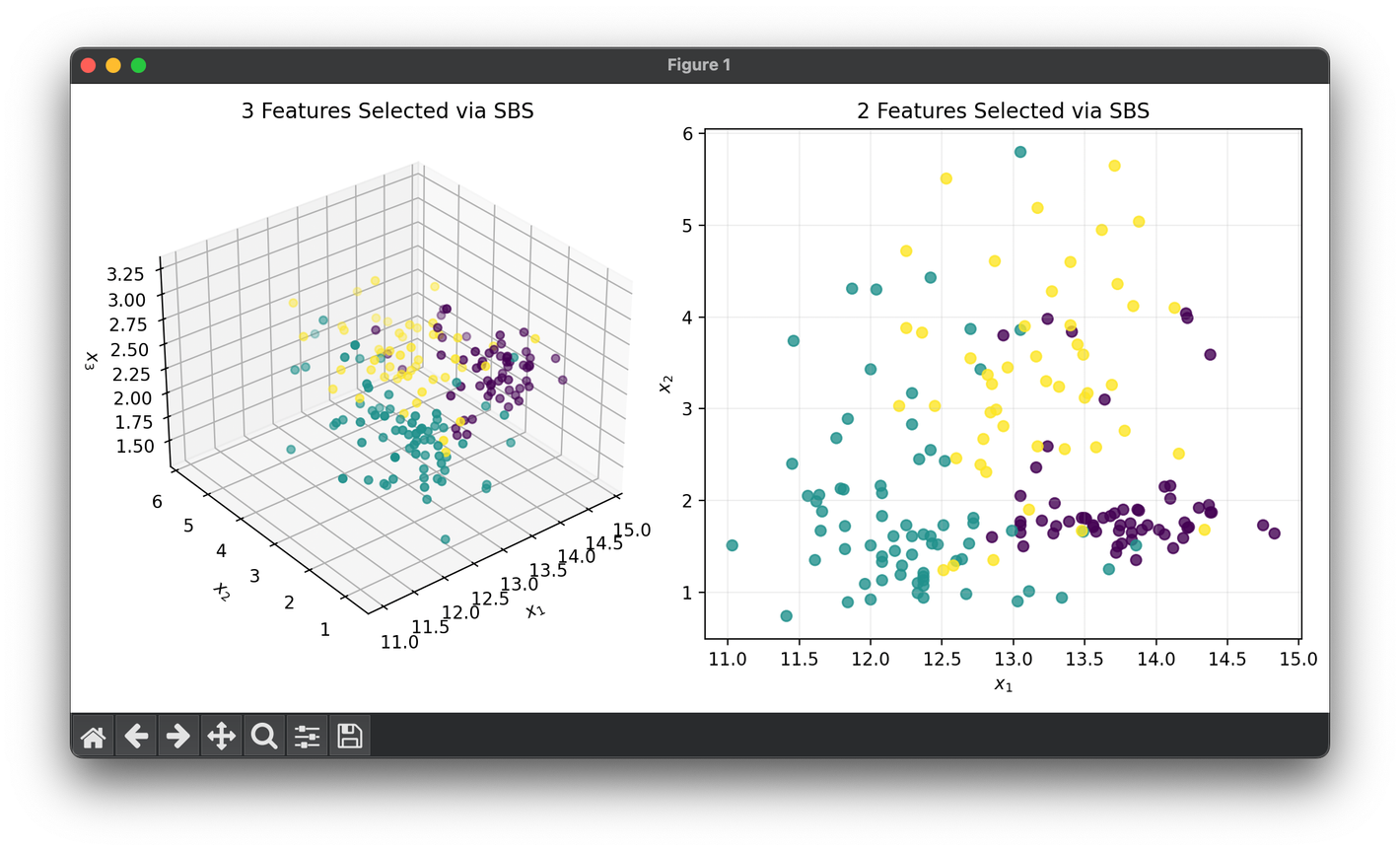
Test on the wine dataset:

from luma.reduction.selection import SBS
from luma.classifier.discriminant import LDAClassifier
from luma.model_selection.fold import StratifiedKFold

from sklearn.datasets import load_wine
import matplotlib.pyplot as plt

X, y = load_wine(return_X_y=True)

model = SBS(estimator=LDAClassifier(),
            n_features=3,
            test_size=0.3,
            cv=10,
            shuffle=True,
            stratify=True,
            fold_type=StratifiedKFold,
            random_state=42)

X_3d = model.fit_transform(X, y)
model.set_params(n_features=2)
X_2d = model.fit_transform(X, y)

fig = plt.figure(figsize=(10, 5))
ax1 = fig.add_subplot(1, 2, 1, projection='3d')
ax2 = fig.add_subplot(1, 2, 2)

ax1.scatter(X_3d[:, 0], X_3d[:, 1], X_3d[:, 2], c=y)
ax1.set_xlabel(r"$x_1$")
ax1.set_ylabel(r"$x_2$")
ax1.set_zlabel(r"$x_3$")
ax1.set_title(f"3 Features Selected via {type(model).__name__}")

ax2.scatter(X_2d[:, 0], X_2d[:, 1], c=y, alpha=0.8)
ax2.set_xlabel(r"$x_1$")
ax2.set_ylabel(r"$x_2$")
ax2.set_title(f"2 Features Selected via {type(model).__name__}")
ax2.grid(alpha=0.2)

plt.tight_layout()
plt.show()

Applications

Sequential Backward Selection is applicable across various domains, including but not limited to:

• Biomedical Signal Processing: For selecting relevant features from high-dimensional biomedical data for disease diagnosis or prognosis.
• Financial Analysis: In portfolio selection or credit scoring, where irrelevant features could lead to misleading predictions or classifications.
• Image Recognition: To select features that are most relevant for image classification tasks, improving accuracy and reducing computational costs.

Strengths and Limitations

Strengths:

• Reduces Overfitting: By eliminating irrelevant features, SBS can help in building models that generalize better to unseen data.
• Improves Model Interpretability: A model with fewer features is easier to understand and interpret.
• Reduces Training Time: Fewer features lead to faster training times, which is beneficial for large datasets.

Limitations:

• Greedy Algorithm: SBS is a greedy algorithm, which means it may not always find the optimal subset of features.
• Evaluation Cost: The process of evaluating the criterion function at each step can be computationally expensive, especially for large datasets.

Advanced Topics

• Integration with Cross-validation: To avoid overfitting and assess the generalizability of the feature subset, SBS can be integrated with cross-validation techniques.
• Hybrid Methods: Combining SBS with other feature selection methods, like Sequential Forward Selection (SFS), can sometimes yield better performance.

References

1. K. P. Soman, R. Loganathan, and V. Ajay, Machine Learning with SVM and other Kernel Methods, PHI Learning Pvt. Ltd., 2009.
2. I. Guyon and A. Elisseeff, "An introduction to variable and feature selection," in Journal of Machine Learning Research, 2003.