Weighted KNN Regression

Introduction

Weighted k-Nearest Neighbors (Weighted KNN) regression is an advanced variation of the basic KNN regression algorithm, which assigns weights to the contributions of the neighbors, allowing closer neighbors to have a greater influence on the prediction. This weighting strategy improves the prediction accuracy by acknowledging that neighbors closer to the query point are more likely to have similar target values than those farther away.

Background and Theory

Principle

The fundamental principle behind Weighted KNN regression is that not all neighbors contribute equally to the prediction of a query point's value. By incorporating a weighting function based on the distance between the query point and its neighbors, Weighted KNN regression accounts for the varying relevance of each neighbor, with closer neighbors deemed more significant than distant ones.

Mathematical Foundation

Given a dataset $D = \{(x_i, y_i)\}_{i=1}^N$ where $x_i$ is a feature vector and $y_i$ is the corresponding target value, the predicted value $\hat{y}_q$ for a query point $x_q$ using Weighted KNN regression is computed as:

Here, $N_k(x_q)$ represents the set of indices of the $k$ nearest neighbors to $x_q$, and $w_i$ denotes the weight assigned to the $i$-th neighbor, which is typically inversely proportional to the distance between the query point $x_q$ and the neighbor $x_i$.

A common choice for the weighting function is:

where $d(x_q, x_i)$ is the distance between $x_q$ and $x_i$, and $p$ is a parameter that controls the influence of distance on the weight. When $p=2$, this corresponds to the inverse of the squared distance.

Choice of Distance Metric

The choice of distance metric (e.g., Euclidean, Manhattan) can significantly affect the performance of Weighted KNN regression, similar to the standard KNN algorithm. The Euclidean distance is the most commonly used metric, defined as:

for feature vectors $x_q$ and $x_i$ in a $d$-dimensional feature space.

Procedural Steps

1. Preprocessing: Normalize or standardize the dataset to ensure that distances are not disproportionately influenced by features on different scales.
2. Distance Calculation: For a query point $x_q$, compute the distance to every training instance.
3. Neighbor Selection: Identify the $k$ nearest neighbors to $x_q$ based on the chosen distance metric.
4. Weight Calculation: Compute weights for these $k$ neighbors, typically inversely proportional to their distances from $x_q$.
5. Weighted Regression: Calculate the weighted average of the target values of the $k$ nearest neighbors to predict $\hat{y}_q$.
6. Postprocessing: Apply any necessary inverse transformations to the predicted value, if preprocessing steps were applied to the target variable.

Implementation

Parameters

• n_neighbors: int, default = 5
  Number of neighbors to be considered close
  

Examples

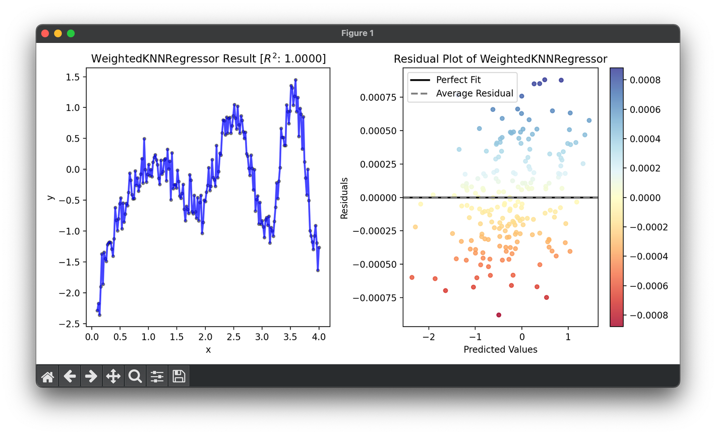
from luma.regressor.neighbors import WeightedKNNRegressor
from luma.metric.regression import RSquaredScore
from luma.visual.evaluation import ResidualPlot

import matplotlib.pyplot as plt
import numpy as np

X = np.linspace(0.1, 4, 200).reshape(-1, 1)
y = (np.cos(X ** 2) * np.log(X)).flatten() + 0.2 * np.random.randn(200)

reg = WeightedKNNRegressor()
reg.fit(X, y)

fig = plt.figure(figsize=(10, 5))
ax1 = fig.add_subplot(1, 2, 1)
ax2 = fig.add_subplot(1, 2, 2)

ax1.scatter(X, y, s=10, c="black", alpha=0.4)
ax1.plot(X, reg.predict(X), lw=2, c="b", alpha=0.7)
ax1.fill_between(X.flatten(), y, reg.predict(X), color="b", alpha=0.1)
ax1.set_xlabel("x")
ax1.set_ylabel("y")
ax1.set_title(
    f"{type(reg).__name__} Result ["
    + r"$R^2$"
    + f": {reg.score(X, y, metric=RSquaredScore):.4f}]"
)

res = ResidualPlot(reg, X, y)
res.plot(ax=ax2, show=True)

Applications

• Real Estate Valuation: More accurately predicting property prices by giving more importance to nearby or similar properties.
• Personalized Recommendation Systems: Recommending items (e.g., movies, products) by weighting user preferences more heavily when they are similar to the query user.
• Healthcare Analytics: Estimating patient outcomes by considering more closely matched patient histories with greater significance.

Strengths and Limitations

Strengths

• Accuracy: Can provide more accurate predictions by emphasizing more relevant neighbors.
• Flexibility: The weighting function and the distance metric can be customized based on the specific requirements of the dataset or application.
• Non-Parametric: Makes no assumptions about the form of the target function, allowing it to model complex relationships.

Limitations

• Parameter Sensitivity: The choice of $k$, the distance metric, and the weighting function can greatly affect performance, requiring careful tuning.
• Scalability: Computationally expensive for large datasets, as it requires calculating distances to all training points for each query.
• Dimensionality: Performance may degrade in high-dimensional spaces due to the curse of dimensionality, making it difficult to find meaningful neighbors.

Advanced Topics

• Cross-Validation for Parameter Tuning: Employing cross-validation techniques to optimize the selection of $k$ and the parameter $p$ in the weighting function.
• Hybrid Models: Combining Weighted KNN with other regression models to leverage the strengths of multiple approaches, potentially improving prediction accuracy and robustness.
• Distance Metric Learning: Learning an optimal distance metric from data to improve the performance of the Weighted KNN algorithm, especially in high-dimensional spaces.

References

1. Dudani, S. A. "The Distance-Weighted k-Nearest-Neighbor Rule." IEEE Transactions on Systems, Man, and Cybernetics, SMC-6.4 (1976): 325-327.
2. Hastie, Trevor, Robert Tibshirani, and Jerome Friedman. The Elements of Statistical Learning. 2nd ed., Springer, 2009.
3. James, Gareth, et al. An Introduction to Statistical Learning: with Applications in R. Springer Texts in Statistics, 2013.