Adaptive KNN Regression

Introduction

Adaptive k-Nearest Neighbors (Adaptive KNN) regression is an enhanced variant of the standard KNN regression algorithm. It adjusts the number of neighbors (k) dynamically based on local density or other criteria, rather than using a fixed 'k' for all predictions. This adaptability allows the algorithm to perform more accurately in regions where data points are sparse or densely packed, optimizing the balance between bias and variance by adapting to the underlying structure of the data.

Background and Theory

Adaptive Strategy

In adaptive KNN regression, the selection of neighbors is based not solely on the closest 'k' instances in the feature space but also on how these instances are distributed. The main idea is to define a neighborhood size that adapts to the local density of points. Regions with a high density of points will use a smaller number of neighbors for predictions, whereas sparse regions will use a larger number. This approach helps in dealing with heterogeneous data densities, improving prediction accuracy especially in areas with few data points.

Mathematical Foundation

The mathematical formulation of adaptive KNN regression extends the standard KNN approach by incorporating a variable neighborhood size. Given a dataset $D = \{(x_i, y_i)\}_{i=1}^N$, the goal remains to predict the target value $y_q$ for a query instance $x_q$. However, instead of using a fixed 'k', an adaptive strategy is employed:

1. Density Estimation: Determine the density around each point, which could be done using methods like kernel density estimation (KDE) or by calculating the distance to the $n$-th nearest neighbor.

2. Neighborhood Adjustment: Adjust the size of the neighborhood based on the density, such that $k = k(x_q)$ varies for different query points $x_q$.

3. Prediction: Compute $y_q$ as an average of the target values of the adjusted number of nearest neighbors, similar to standard KNN but with a variable $k$:

   $y_q = \frac{1}{k(x_q)} \sum_{i \in N_{k(x_q)}(x_q)} y_i$

Choice of Adaptivity Criteria

The method of adjusting 'k' can vary, with common criteria including:

• Local density: Use measures of local point density to decide on 'k'.
• Distance thresholds: Set a maximum distance within which neighbors must fall, adjusting 'k' accordingly.

Procedural Steps

1. Preprocessing: Standardize the dataset to ensure that distance metrics are applied uniformly across features.
2. Density Estimation: For each point in the dataset, estimate the local density or compute distances to determine how 'k' should be adjusted.
3. Distance Calculation: For a given query instance, calculate the distance to all points in the training set.
4. Adaptive Neighbor Selection: Determine the optimal number of neighbors based on the pre-determined adaptivity criteria.
5. Regression: Calculate the average target value of the selected neighbors.
6. Postprocessing: Apply any necessary inverse transformations on the predicted values.

Implementation

Parameters

• n_density: int, default = 10
  Number of nearest neighbors to estimate the local density
  
• min_neighbors: int, default = 5
  Minimum number of neighbors to be considered for averaging
  
• max_neighbors: int, default = 20
  Maximum number of neighbors to be considered
  

Exmaples

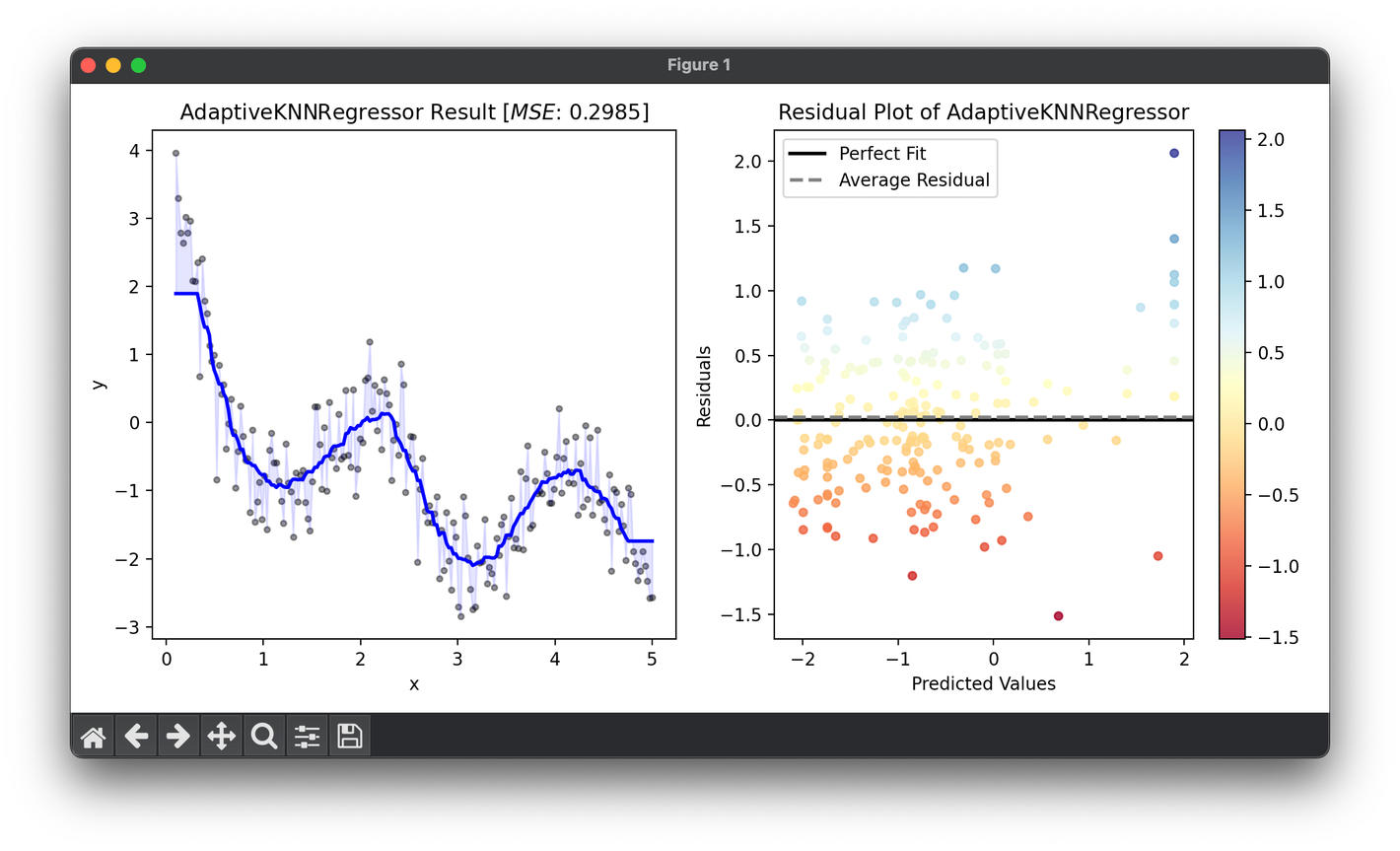
from luma.regressor.neighbors import AdaptiveKNNRegressor
from luma.model_selection.search import GridSearchCV
from luma.metric.regression import MeanSquaredError
from luma.visual.evaluation import ResidualPlot

import matplotlib.pyplot as plt
import numpy as np

X = np.linspace(0.1, 5, 200).reshape(-1, 1)
y = (np.cos(3 * X) - np.log(X)).flatten() + 0.5 * np.random.randn(200)

param_grid = {
    "n_density": range(5, 20)
}

grid = GridSearchCV(
    estimator=AdaptiveKNNRegressor(),
    param_grid=param_grid,
    cv=5,
    metric=MeanSquaredError,
    maximize=False,
    shuffle=True,
    random_state=42,
)

grid.fit(X, y)
print(grid.best_params, grid.best_score)
reg = grid.best_model

fig = plt.figure(figsize=(10, 5))
ax1 = fig.add_subplot(1, 2, 1)
ax2 = fig.add_subplot(1, 2, 2)

ax1.scatter(X, y, s=10, c="black", alpha=0.4)
ax1.plot(X, reg.predict(X), lw=2, c="b")
ax1.fill_between(X.flatten(), y, reg.predict(X), color="b", alpha=0.1)
ax1.set_xlabel("x")
ax1.set_ylabel("y")
ax1.set_title(
    f"{type(reg).__name__} Result ["
    + r"$MSE$"
    + f": {reg.score(X, y, metric=MeanSquaredError):.4f}]"
)

res = ResidualPlot(reg, X, y)
res.plot(ax=ax2, show=True)

Applications

• Environmental Modeling: More accurately predicting phenomena like pollution levels or temperature in regions with varying data point densities.
• Healthcare: Improving patient diagnosis by adapting to the varied distribution of disease characteristics across populations.
• Financial Forecasting: Enhancing stock price predictions in markets with heterogeneous trading volumes.

Strengths and Limitations

Strengths

• Improved Accuracy: Adapts to local data characteristics, offering potentially higher accuracy especially in sparse regions.
• Versatility: Can be fine-tuned for various applications and data densities.
• Non-parametric: Retains the non-parametric nature of KNN, requiring no assumption about the data distribution.

Limitations

• Complexity: Determining the best method for adjusting 'k' can add complexity.
• Computationally Intensive: Especially in the density estimation step, which can be costly for large datasets.
• Sensitive to Feature Scale: Like standard KNN, it is sensitive to the scaling of data features, necessitating careful preprocessing.

Advanced Topics

• Automated Parameter Tuning: Using cross-validation to automatically determine the best parameters for density estimation and neighborhood size adjustment.
• Integration with Machine Learning Pipelines: Incorporating adaptive KNN regression into larger machine learning workflows for tasks like feature engineering and model stacking.
• Hybrid Approaches: Combining adaptive KNN with other regression techniques to leverage the strengths of multiple approaches.

References

1. Samworth, Richard J. "Optimal weighted nearest neighbour classifiers." The Annals of Statistics, vol. 40, no. 5, 2012, pp. 2733-2763.
2. Hastie, Trevor, et al. The Elements of Statistical Learning: Data Mining, Inference, and Prediction. 2nd ed., Springer, 2009.
3. Loader, Clive. Local Regression and Likelihood. Springer, 1999.