Polynomial Regression

Introduction

Polynomial regression is a statistical technique that expands the capabilities of linear regression by modeling the relationship between the independent variable $x$ and the dependent variable $y$ as an $n$-th degree polynomial. It provides a way to model a nonlinear relationship through a linear model, by introducing polynomial features, thereby accommodating a broader range of data structures.

Background and Theory

Polynomial Features and Vandermonde Matrix

Polynomial regression can be implemented by transforming the original input features into polynomial features. This process involves generating every combination of features raised to every power up to the $n$ th degree. For a single independent variable $x$, the polynomial features would be $x, x^2, x^3, \ldots, x^n$. This transformation of the input variable into a set of polynomial features is represented by the Vandermonde matrix.

A Vandermonde matrix for a single independent variable $x$ with $m$ observations and a polynomial degree of $n$ is structured as follows:

This matrix is used to transform the single-dimensional input $x$ into a multi-dimensional feature space, where linear regression techniques can then be applied.

Polynomial Regression Model

Given the Vandermonde matrix $\mathbf{V}$ and a response vector $\mathbf{y}$ with $m$ observations, the polynomial regression model can be expressed as:

where:

• $\mathbf{y}$ is the vector of observed values of the dependent variable,
• $\mathbf{V}$ is the Vandermonde matrix of transformed polynomial features,
• $\boldsymbol{\beta}$ is the vector of coefficients $[\beta_0, \beta_1, \cdots, \beta_n]^T$,
• $\boldsymbol{\epsilon}$ represents the vector of errors or residuals.

Derivation of the Normal Equation

The normal equation is derived from the principle of least squares, which aims to minimize the sum of squared residuals $RSS$ between the observed values $y$ and the values predicted by the model $\hat{y}$.

Given the model equation in matrix form as $\mathbf{y} = \mathbf{V}\boldsymbol{\beta} + \boldsymbol{\epsilon}$, where $\mathbf{V}$ is the Vandermonde matrix of polynomial features and $\mathbf{y}$ is the vector of observed values, the RSS is defined as:

To find the minimum of $RSS$, we take its derivative with respect to $\boldsymbol{\beta}$ and set it to zero. This process involves the following steps:

1. Expand the RSS equation:

   $RSS = \mathbf{y}^T\mathbf{y} - \mathbf{y}^T\mathbf{V}\boldsymbol{\beta} - \boldsymbol{\beta}^T\mathbf{V}^T\mathbf{y} + \boldsymbol{\beta}^T\mathbf{V}^T\mathbf{V}\boldsymbol{\beta}$

2. Take the derivative of RSS with respect to $\boldsymbol{\beta}$:

   $\frac{\partial RSS}{\partial \boldsymbol{\beta}} = -2\mathbf{V}^T\mathbf{y} + 2\mathbf{V}^T\mathbf{V}\boldsymbol{\beta}$

3. Set the derivative to zero and solve for $\boldsymbol{\beta}$:

   $\mathbf{V}^T\mathbf{V}\boldsymbol{\beta} = \mathbf{V}^T\mathbf{y}$
   $\boldsymbol{\beta} = (\mathbf{V}^T\mathbf{V})^{-1}\mathbf{V}^T\mathbf{y}$

This final equation, $\boldsymbol{\beta} = (\mathbf{V}^T\mathbf{V})^{-1}\mathbf{V}^T\mathbf{y}$, is known as the normal equation. It provides a direct method to compute the coefficients $\boldsymbol{\beta}$ that minimize the $RSS$, and thus, the error between the predicted and observed values.

Detailed Computation Steps

Normal Equation Computation

1. Generate the Vandermonde Matrix $\mathbf{V}$ for your data.
2. Compute $\mathbf{V}^T\mathbf{V}$: Multiply the transpose of $\mathbf{V}$ by $\mathbf{V}$.
3. Compute $(\mathbf{V}^T\mathbf{V})^{-1}$: Find the inverse of the matrix obtained in step 2.
4. Compute $\mathbf{V}^T\mathbf{y}$: Multiply the transpose of $\mathbf{V}$ by the response vector $\mathbf{y}$.
5. Calculate $\boldsymbol{\beta}$: Multiply the matrix from step 3 by the vector obtained in step 4.

Polynomial Feature Generation

To generate polynomial features and the Vandermonde matrix in practice, one often uses computational tools or libraries that automate this process, especially for datasets with multiple features and higher-degree polynomials.

Implementation

Parameters

• deg: int, default = 2
  Degree of a polynomial function
  
• alpha: float, default = 1.0
  Regularization strength
  
• l1_ratio: float, default = 0.5
  Balancing parameter between L1 and L2 regularization
  

Examples

from luma.regressor.poly import PolynomialRegressor
from luma.model_selection.search import RandomizedSearchCV
from luma.metric.regression import RSquaredScore
from luma.visual.evaluation import ResidualPlot

import matplotlib.pyplot as plt
import numpy as np

X = np.linspace(0.1, 3, 200).reshape(-1, 1)
y = (np.cos(X**2) * np.log(X)).flatten() + 0.2 * np.random.randn(200)

param_dist = {
    "deg": range(2, 10),
    "alpha": np.logspace(-3, 3, 5),
    "l1_ratio": np.linspace(0, 1, 5),
    "regularization": ["l1", "l2", "elastic-net"],
}

rand = RandomizedSearchCV(
    estimator=PolynomialRegressor(),
    param_dist=param_dist,
    max_iter=100,
    cv=5,
    metric=RSquaredScore,
    maximize=True,
    refit=True,
    shuffle=True,
    random_state=42,
)
rand.fit(X, y)
print(rand.best_params, rand.best_score)
reg = rand.best_model

est_func = r""
for i, coef in enumerate(reg.coef_):
    est_func = f"+({coef:.2f})x^{i}" + est_func
print(est_func)

fig = plt.figure(figsize=(10, 5))
ax1 = fig.add_subplot(1, 2, 1)
ax2 = fig.add_subplot(1, 2, 2)

ax1.scatter(X, y, s=10, c="black", alpha=0.4)
ax1.plot(X, reg.predict(X), lw=2, c="b", alpha=0.7, label="Predicted Plot")
ax1.fill_between(X.flatten(), y, reg.predict(X), color="b", alpha=0.1)
ax1.set_xlabel("x")
ax1.set_ylabel("y")
ax1.set_title(
    f"{type(reg).__name__} Result ["
    + r"$R^2$"
    + f": {reg.score(X, y, metric=RSquaredScore):.4f}]"
)
ax1.legend()
ax1.grid(alpha=0.2)

res = ResidualPlot(reg, X, y)
res.plot(ax=ax2, show=True)

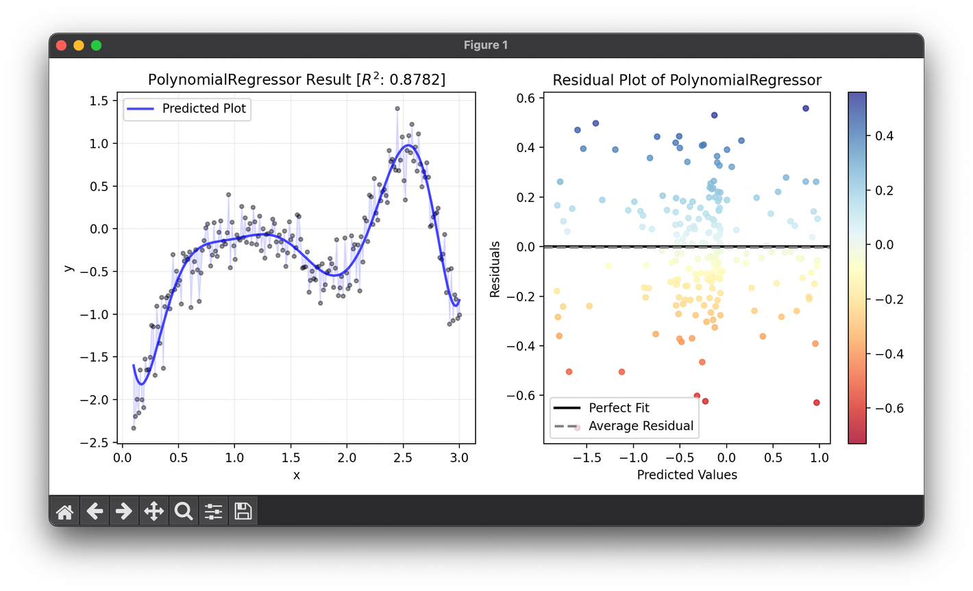
• Predicted plot:
  $y=1.48x^7-17.86x^6+88.24x^5-231.27x^4+347.48x^3-300.51x^2+139.62x-27.29$

Applications

Polynomial regression is widely used in fields such as:

• Economics: For modeling economic growth patterns or the impact of policy changes.
• Engineering: In signal processing and the analysis of stress-strain curves.
• Environmental Science: Modeling the relationship between environmental factors and biological responses.

Strengths and Limitations

Strengths

• Flexibility: Can model complex, nonlinear relationships between dependent and independent variables.
• Simplicity: Despite being able to fit nonlinear patterns, it remains a linear model, making it relatively straightforward to analyze and interpret.

Limitations

• Overfitting: Higher-degree polynomials can lead to overfitting the training data, capturing noise rather than the underlying trend.
• Extrapolation: Polynomial regression models can exhibit extreme behavior outside the range of the training data, making predictions less reliable.
• Computation: The inversion of $\mathbf{V}^T\mathbf{V}$ can be computationally expensive and numerically unstable for high-degree polynomials or large datasets.