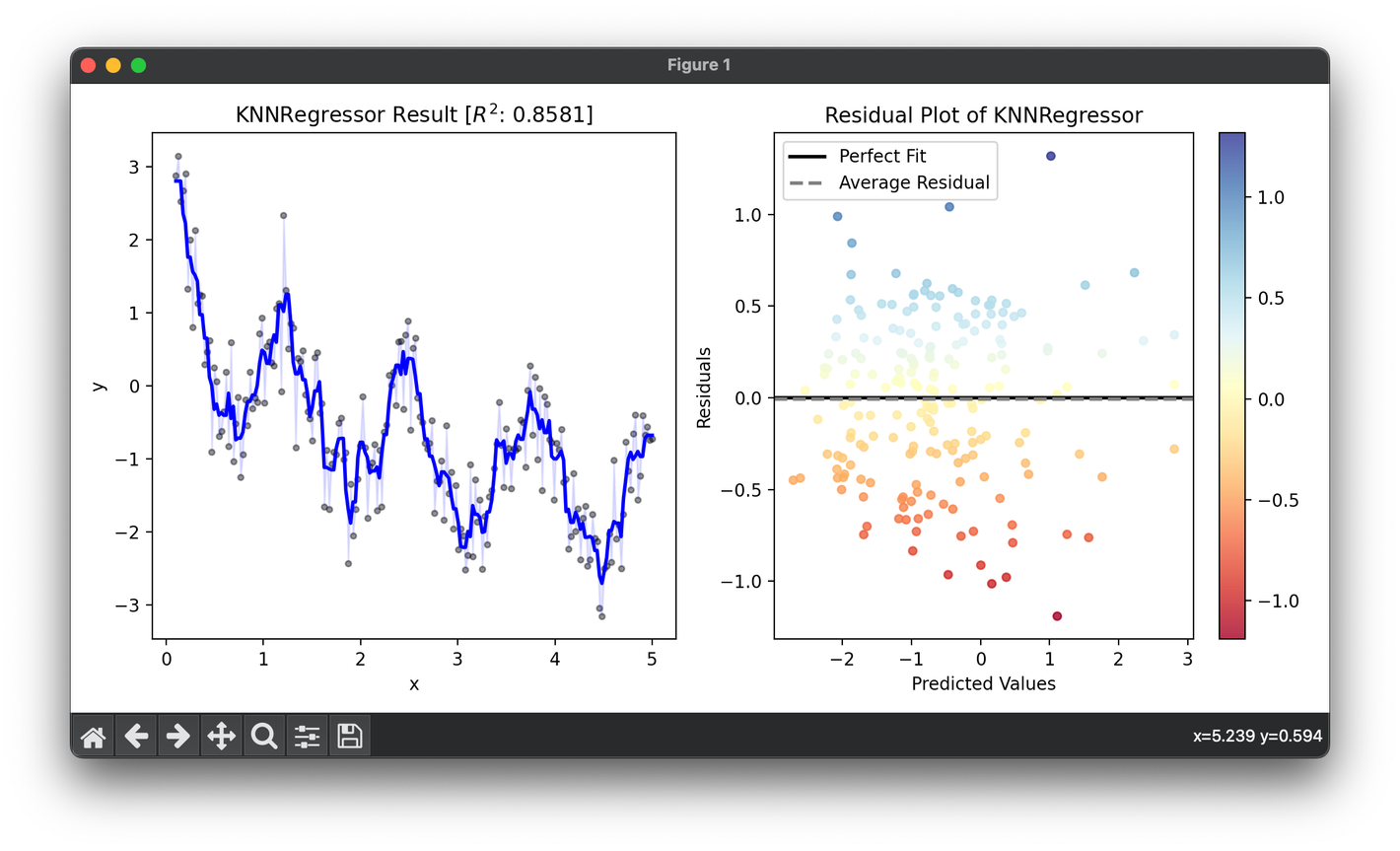
K-Nearest Neighbors Regressor

Introduction

The k-Nearest Neighbors (KNN) regressor is a type of instance-based learning, or lazy learning, where the function is only approximated locally and all computation is deferred until function evaluation. It is one of the simplest machine learning algorithms, based on supervised learning technique. The KNN regressor estimates the value of a given point based on the values of the nearest points in the training dataset. Unlike its classification counterpart, which predicts a class label, the KNN regressor predicts a continuous value. The simplicity of the KNN regressor, along with its relatively high accuracy in many cases, makes it a widely used algorithm for regression tasks.

Background and Theory

Principle

The KNN regressor operates on a simple principle: it calculates the distance (usually Euclidean) between the query instance and all the instances in the training set, selects the nearest 'k' instances from the training data, and then averages the target values of these nearest neighbors as the prediction for the query instance.

Mathematical Foundation

Given a dataset $D = \{(x_i, y_i)\}_{i=1}^N$ where $x_i$ is a vector in a multidimensional feature space $\mathbb{R}^d$ and $y_i$ is the target value (real number) associated with $x_i$. The goal of KNN regression is to predict the target value $y_q$ for a query instance $x_q$. This is done as follows:

1. Distance Metric: Calculate the distance between $x_q$ and every instance $x_i$ in the dataset. Although Euclidean distance is the most common metric, other distances like Manhattan, Minkowski, or Hamming can be used depending on the nature of the data.
   Euclidean distance between two points $x_q$ and $x_i$ in $\mathbb{R}^d$ is defined as:

   $d(x_q, x_i) = \sqrt{\sum_{j=1}^d (x_{qj} - x_{ij})^2}$

2. Selecting Neighbors: Identify the 'k' instances in the training data that are nearest to $x_q$ based on the distance metric.

3. Prediction: Compute the output for $x_q$ by averaging the target values $y_i$ of the nearest neighbors.

   $y_q = \frac{1}{k} \sum_{i \in N_k(x_q)} y_i$

   where $N_k(x_q)$ is the set of indices of the 'k' nearest neighbors to $x_q$.

Choice of $k$

The choice of the parameter 'k' is critical in KNN algorithms. A smaller value of 'k' can make the algorithm sensitive to noise in the data, while a larger 'k' makes it computationally expensive and possibly overshoots the small but important patterns in the data.

Procedural Steps

1. Preprocessing: Normalize or standardize the data if the features are on very different scales or types to ensure distance metrics are meaningful.
2. Distance Calculation: Compute the distance between the query instance and all instances in the training dataset.
3. Neighbor Selection: Sort the distances and select the top 'k' instances closest to the query instance.
4. Regression: Average the target values of these 'k' nearest neighbors.
5. Postprocessing: If any data postprocessing steps are necessary (e.g., inverse transformations applied during preprocessing), perform them on the predicted value.

Implementation

Parameters

• n_neighbors: int, default = 5
  Number of neighbors to be considered close
  

Examples

from luma.regressor.neighbors import KNNRegressor
from luma.model_selection.search import GridSearchCV
from luma.metric.regression import RSquaredScore
from luma.visual.evaluation import ResidualPlot

import matplotlib.pyplot as plt
import numpy as np

X = np.linspace(0.1, 5, 200).reshape(-1, 1)
y = (np.cos(5 * X) - np.log(X)).flatten() + 0.5 * np.random.randn(200)

param_grid = {
    "n_neighbors": range(2, 20)
}

grid = GridSearchCV(
    estimator=KNNRegressor(),
    param_grid=param_grid,
    cv=5,
    metric=RSquaredScore,
    maximize=True,
    shuffle=True,
    random_state=42,
)

grid.fit(X, y)
print(grid.best_params, grid.best_score)
reg = grid.best_model

fig = plt.figure(figsize=(10, 5))
ax1 = fig.add_subplot(1, 2, 1)
ax2 = fig.add_subplot(1, 2, 2)

ax1.scatter(X, y, s=10, c="black", alpha=0.4)
ax1.plot(X, reg.predict(X), lw=2, c="b")
ax1.fill_between(X.flatten(), y, reg.predict(X), color="b", alpha=0.1)
ax1.set_xlabel("x")
ax1.set_ylabel("y")
ax1.set_title(
    f"{type(reg).__name__} Result ["
    + r"$R^2$"
    + f": {reg.score(X, y, metric=RSquaredScore):.4f}]"
)

res = ResidualPlot(reg, X, y)
res.plot(ax=ax2, show=True)

Applications

• Real Estate: Estimating the value of a property based on the characteristics and values of nearby properties.
• Finance: Predicting stock prices based on the historical prices of the nearest neighbors.
• Healthcare: Estimating patient health metrics based on similar patients' records.
• Energy Consumption: Predicting energy consumption of a household based on nearby similar households.

Strengths and Limitations

Strengths

• Simplicity: Easy to understand and implement.
• Flexibility: Can work with any number of features and is applicable to various types of data.
• Non-parametric: Makes no assumptions about the underlying data distribution.

Limitations

• Scalability: Computationally expensive as the dataset grows, since it requires calculating the distance to every point in the dataset.
• High Memory Requirement: Needs to store the entire dataset.
• Sensitivity to Irrelevant Features: Performance can degrade with irrelevant features because all features contribute equally to the distance computation.

Advanced Topics

• Weighted KNN: Instead of giving equal weight to all neighbors, weights can be assigned inversely proportional to the distance. Closer neighbors will have more influence on the output.
• Feature Selection: Techniques to select the most relevant features can improve performance and computational efficiency.
• Distance Metric Customization: Exploring different distance metrics tailored to the specific characteristics of the dataset can yield better results.

References

1. Altman, N. S. "An Introduction to Kernel and Nearest-Neighbor Nonparametric Regression." The American Statistician, vol. 46, no. 3, 1992, pp. 175-185.
2. James, Gareth, et al. An Introduction to Statistical Learning: with Applications in R. Springer, 2013.
3. Mitchell, Tom M. Machine Learning. McGraw Hill, 1997.