Bayesian Ridge Regression

Introduction

Bayesian Ridge Regression extends traditional ridge regression by incorporating Bayesian inference, offering a probabilistic approach to regression modeling. This method not only estimates the regression coefficients but also assesses the uncertainty in these estimates, providing a comprehensive view of the model's parameters. Through Bayesian techniques, this regression model applies prior distributions to the coefficients, updating these beliefs in light of observed data to compute posterior distributions. This document explores the mathematical underpinnings, applications, and nuances of Bayesian Ridge Regression.

Theoretical Framework

Ridge Regression Overview

In ridge regression, the objective is to minimize the penalized residual sum of squares, with a penalty on the L2-norm of the coefficients:

Here, $\lambda$ denotes the regularization strength, influencing the degree of shrinkage applied to the coefficients.

Bayesian Perspective on Regression

Bayesian inference treats model parameters as random variables, introducing prior distributions over these parameters. The essence of Bayesian regression lies in updating our knowledge about these parameters (posterior distribution) based on observed data and prior beliefs.

Mathematical Formulation

Likelihood Function

Assuming the data $\{y_i, X_i\}_{i=1}^n$ and a linear model $y = X\beta + \epsilon$, with $\epsilon \sim \mathcal{N}(0, \sigma^2I)$, the likelihood of observing $y$ given $X$ and $\beta$ is:

Prior Distributions

Priors over the regression coefficients $\beta$ and the precision $\alpha = 1/\sigma^2$ (inverse of variance) are typically chosen to be Gaussian and Gamma distributions, respectively:

• For coefficients: $\beta \sim \mathcal{N}(0, \lambda^{-1}I)$
• For precision: $\alpha \sim \text{Gamma}(a, b)$

These priors encapsulate our beliefs about the parameters before observing the data.

Posterior Distribution

The posterior distribution of $\beta$ given the data and hyperparameters ($\lambda$, $a$, $b$) is derived using Bayes' theorem:

Given the Gaussian likelihood and prior, the posterior distribution of $\beta$ is also Gaussian, with updated mean and variance that depend on the data and the value of $\alpha$.

Estimation of Coefficients

The coefficients are estimated by maximizing the posterior distribution (MAP estimation), which can be analytically solved due to the conjugacy of the prior and likelihood in the Gaussian case:

The precision $\alpha$ and regularization parameter $\lambda$ can be estimated using empirical Bayes methods, where they are iteratively updated based on the data.

Implementation

Parameters

• alpha_init: float, default = None
  Initial value for the precision of the distribution of noise
  
• lambda_init: float, default = None
  Initial value for the precision of the distribution of weights
  

Examples

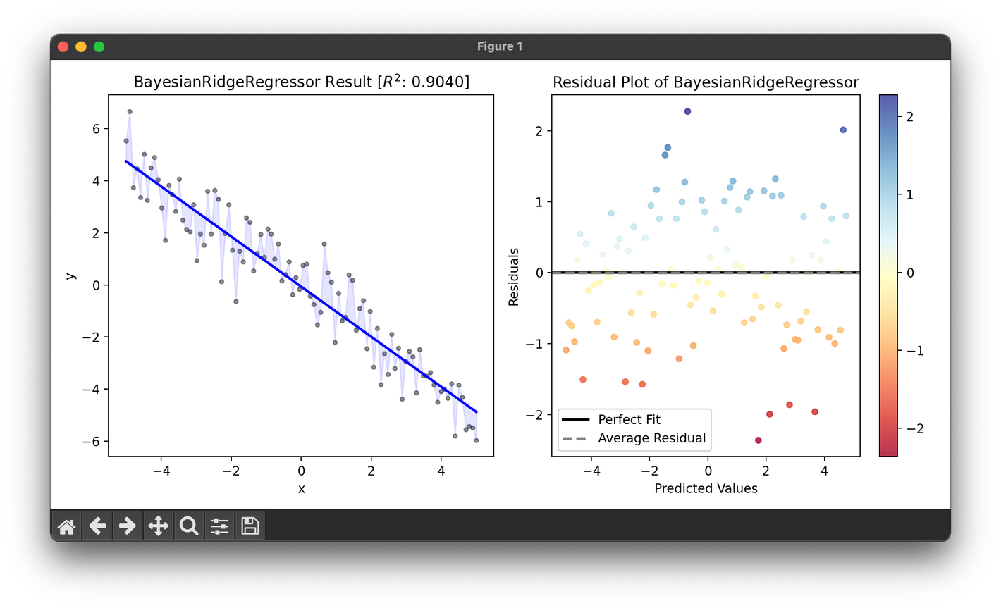
from luma.regressor.linear import BayesianRidgeRegressor
from luma.model_selection.search import GridSearchCV
from luma.metric.regression import RSquaredScore
from luma.visual.evaluation import ResidualPlot

import matplotlib.pyplot as plt
import numpy as np

X = np.linspace(-5, 5, 100).reshape(-1, 1)
y = (0.5 * np.cos(X) - X).flatten() + np.random.randn(100)

param_grid = {
    "alpha_init": np.logspace(-5, -1, 5),
    "lambda_init": np.logspace(-5, -1, 5),
}

grid = GridSearchCV(
    estimator=BayesianRidgeRegressor(),
    param_grid=param_grid,
    cv=5,
    metric=RSquaredScore,
    maximize=True,
    shuffle=True,
    random_state=42,
)
grid.fit(X, y)
print(grid.best_params, grid.best_score)
reg = grid.best_model

fig = plt.figure(figsize=(10, 5))
ax1 = fig.add_subplot(1, 2, 1)
ax2 = fig.add_subplot(1, 2, 2)

ax1.scatter(X, y, s=10, c="black", alpha=0.4)
ax1.plot(X, reg.predict(X), lw=2, c="b")
ax1.fill_between(X.flatten(), y, reg.predict(X), color="b", alpha=0.1)
ax1.set_xlabel("x")
ax1.set_ylabel("y")
ax1.set_title(
    f"{type(reg).__name__} Result ["
    + r"$R^2$"
    + f": {reg.score(X, y, metric=RSquaredScore):.4f}]"
)

res = ResidualPlot(reg, X, y)
res.plot(ax=ax2, show=True)

Applications

Bayesian Ridge Regression's ability to quantify uncertainty makes it invaluable in fields requiring risk assessment, such as:

• Finance: Estimating stock returns with confidence intervals.
• Bioinformatics: Predicting gene expression levels with uncertainty measures.
• Environmental Science: Forecasting climate variables, offering a range of possible outcomes.

Strengths and Limitations

Strengths

• Probabilistic Insights: Provides a full probabilistic model of the data, including uncertainty in the estimates.
• Incorporation of Prior Knowledge: Enables the inclusion of prior knowledge through the choice of prior distributions.

Limitations

• Computational Complexity: The computation of posterior distributions, especially in high-dimensional spaces, can be resource-intensive.
• Hyperparameter Tuning: The choice of hyperparameters for the prior distributions can significantly affect model performance and requires careful selection, often through empirical Bayes or cross-validation methods.

Conclusion

Bayesian Ridge Regression represents a robust approach to regression analysis, offering not only point estimates for regression coefficients but also a comprehensive assessment of uncertainty. By employing Bayesian methods, it allows for the incorporation of prior knowledge and provides a deeper understanding of the model's parameters, making it a powerful tool for predictive modeling across various disciplines.