Kernel Ridge Regression

Introduction

Kernel Ridge Regression (KRR) is an advanced machine learning algorithm that combines ridge regression's regularization techniques with the kernel trick to enable efficient learning in high-dimensional feature spaces. It's particularly effective for non-linear regression tasks, providing a way to capture complex relationships in data without explicitly computing the high-dimensional feature transformations. This document delves into the fundamentals, mathematical underpinnings, and applications of KRR, offering a comprehensive overview suited for a wide range of audiences interested in machine learning and statistical modeling.

Theoretical Framework

Ridge Regression Recap

Ridge regression is a linear regression technique that introduces an L2 penalty on the size of coefficients to reduce model complexity and prevent overfitting. The optimization problem in ridge regression is given by:

where $\lambda$ is the regularization parameter, and $n$ and $p$ are the number of observations and predictors, respectively.

The Kernel Trick

The kernel trick is a method used in machine learning to implicitly map input features into high-dimensional feature spaces without explicitly performing the transformation. It relies on the fact that many algorithms can be expressed in terms of dot products between data points. A kernel function computes the dot product in the transformed space without the actual computation of coordinates in that space, thus enabling efficient computations.

Kernel Ridge Regression

KRR applies the kernel trick to ridge regression, allowing it to learn non-linear relationships. The regression function is modeled as:

where $k(x, x_i)$ is the kernel function, $\alpha_i$ are the coefficients to be learned, and $b$ is the bias term. The commonly used kernel functions include the linear, polynomial, and radial basis function (RBF) kernels.

Mathematical Formulation

Optimization Problem

The objective function in KRR is formulated as minimizing the squared loss with an L2 penalty on the coefficients, expressed in terms of the kernel function:

where $K$ is the kernel matrix with $K_{ij} = k(x_i, x_j)$, and $\lambda$ is the regularization parameter.

Solution

The solution to the KRR optimization problem involves solving a system of linear equations:

where $\mathbf{I}$ is the identity matrix, and $\mathbf{y}$ is the vector of target values. The solution $\alpha$ can be found by inverting the matrix $(\mathbf{K} + \lambda \mathbf{I})$.

Implementation

Parameters

• alpha: float, default = 1.0
  Regularization strength
  
• deg: int, default = 2
  Degree for polynomial kernel
  
• gamma: float, default = 1.0
  Scaling factor for RBF, $\tanh$, Laplacian kernels
  
• coef: float, default = 1.0
  Base coefficient for linear and polynomial kernels
  
• kernel: FuncType, default = ‘rbf’
  Kernel function type
  

Examples

from luma.regressor.linear import KernelRidgeRegressor
from luma.model_selection.search import RandomizedSearchCV
from luma.metric.regression import MeanSquaredError
from luma.visual.evaluation import ResidualPlot

import matplotlib.pyplot as plt
import numpy as np

X = np.linspace(-3, 3, 100).reshape(-1, 1)
y = (np.sin(X ** 2) - X).flatten() + 0.5 * np.random.randn(100)

param_dist = {"alpha": np.logspace(-3, 3, 5),
              "deg": range(2, 10),
              "gamma": np.logspace(-3, 1, 5),
              "kernel": ["poly", "rbf", "tanh", "lap"]}

rand = RandomizedSearchCV(estimator=KernelRidgeRegressor(),
                          param_dist=param_dist,
                          max_iter=100,
                          cv=5,
                          metric=MeanSquaredError,
                          maximize=False,
                          refit=True,
                          shuffle=True,
                          random_state=42)
rand.fit(X, y)
print(rand.best_params, rand.best_score)
reg = rand.best_model

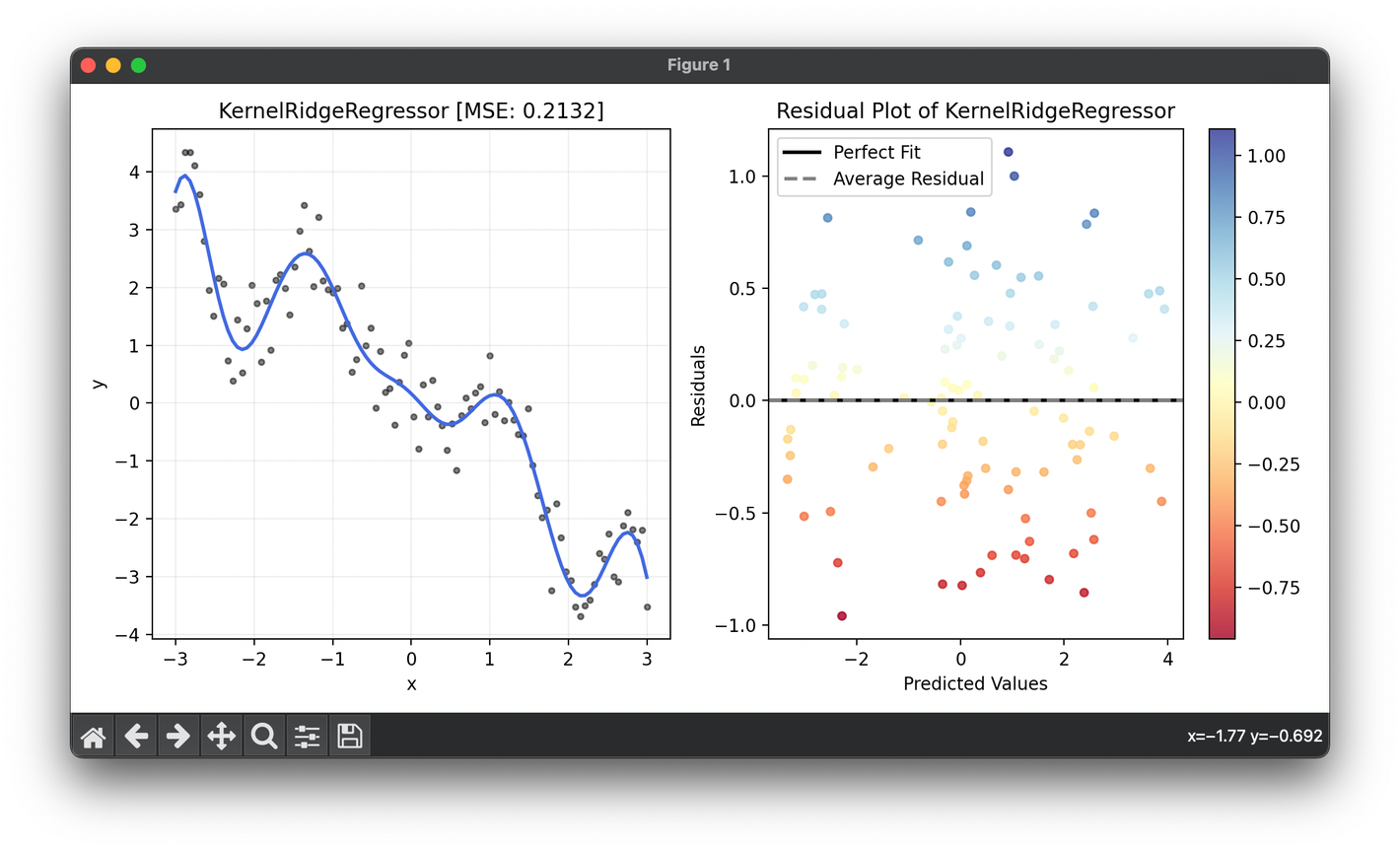
fig = plt.figure(figsize=(10, 5))
ax1 = fig.add_subplot(1, 2, 1)
ax2 = fig.add_subplot(1, 2, 2)

ax1.scatter(X, y, s=10, c="black", alpha=0.5, label=r"y=x+\epsilon")
ax1.plot(X, reg.predict(X), lw=2, c="royalblue")
ax1.set_xlabel("x")
ax1.set_ylabel("y")
ax1.set_title(f"{type(reg).__name__} [MSE: {reg.score(X, y):.4f}]")
ax1.grid(alpha=0.2)

res = ResidualPlot(reg, X, y)
res.plot(ax=ax2, show=True)

Applications

KRR is versatile and applicable in various domains, including:

• Bioinformatics: For predicting genetic traits or the effects of potential drug compounds.
• Finance: In forecasting stock prices or economic indicators where non-linear patterns are prevalent.
• Image and Signal Processing: For tasks like image denoising, where capturing complex patterns is crucial.

Strengths and Limitations

Strengths

• Flexibility: Can model complex, non-linear relationships through the choice of the kernel.
• Regularization: Incorporates regularization automatically, helping to prevent overfitting.

Limitations

• Scalability: The need to store and invert a large kernel matrix makes KRR computationally intensive for large datasets.
• Parameter Selection: Choosing the right kernel and regularization parameter $\lambda$ can be challenging and requires cross-validation.

Advanced Topics

Hyperparameter Optimization

Selecting optimal values for $\lambda$ and any parameters associated with the chosen kernel function is crucial for model performance. Techniques like grid search and random search, often coupled with cross-validation, are employed to find the best hyperparameters.

Kernel Selection

The choice of kernel function has a significant impact on the model's ability to capture complex patterns. Experimentation with different kernels and understanding the underlying data distribution are essential steps in the modeling process.

Conclusion

Kernel Ridge Regression extends the capabilities of traditional ridge regression to handle non-linear relationships through the use of kernel functions. Despite its computational challenges, it remains a powerful tool for regression tasks where linear models fall short. With careful selection of hyperparameters and kernels, KRR can uncover intricate patterns in data, making it a valuable technique in the arsenal of machine learning practitioners.