Decision Tree Regression

Decision Tree Regression is a versatile machine learning algorithm used for predicting a continuous quantity. Unlike its counterpart used for classification tasks, the regression decision tree aims to predict a quantitative response. This documentation provides an in-depth look at the decision tree regression algorithm, emphasizing various criteria used for splitting nodes. We cover its theoretical background, mathematical formulations, procedural steps, applications, strengths, limitations, and advanced topics.

Introduction

Decision tree regression operates by splitting the data into distinct subsets based on certain criteria. The tree is built by splitting the dataset into branches, which represent decisions or conditions leading to different outcomes. In the context of regression, the decision at each node is made with the goal of reducing variance within each node, leading to a prediction that is as accurate as possible.

Background and Theory

Splitting Criteria

For regression tasks, decision trees primarily use variance reduction as the criterion for splitting. The goal is to find the feature and threshold that result in the highest decrease in variance for the target variable among the resulting subsets. The most commonly used criteria for regression trees are:

1. Variance Reduction: It is the most straightforward approach, where the variance of the target variable is calculated before and after the split. The feature and threshold that maximize the reduction in variance are chosen for the split.
2. Mean Squared Error (MSE): This criterion looks for a split that minimizes the MSE across the branches that result from the split. MSE is a measure of the average squared difference between the observed actual outcomes and the outcomes predicted by the model.
3. Mean Absolute Error (MAE): Similar to MSE, MAE minimizes the absolute difference between the actual and predicted values. While MSE gives higher weight to larger errors, MAE treats all errors uniformly.

Mathematically, for a given node $t$, let $S_t$ be the set of samples at that node. The variance before the split is given by:

where $|S_t|$ is the number of samples in node $t$, $y_i$ is the target value of sample $i$, and $\bar{y}_t$ is the mean target value in $S_t$.

The improvement in variance, or variance reduction, for a split that divides $S_t$ into two subsets $S_{t,left}$ and $S_{t,right}$ is given by:

The goal is to maximize $\Delta\text{Var}$.

Tree Construction

1. Start at the root node with the entire dataset.
2. Select the best split according to the chosen criterion (e.g., variance reduction).
3. Split the dataset into two subsets using the chosen feature and threshold.
4. Repeat the process for each child node until a stopping criterion is met (e.g., maximum depth, minimum samples at a node, or no further reduction in variance is possible).
5. Prediction: The prediction for a leaf node is the average target value of the samples in that node.

Implementation

Parameters

• max_depth: int, default = 10
  Maximum depth of the tree
  
• min_samples_split: int, default = 2
  Minimum samples required to split a node
  
• min_samples_leaf: int, default = 1
  Minimum samples required to be at a leaf node
  
• max_features: int, default = None
  Number of features to consider
  
• min_variance_decrease: float, default = 0.0
  Minimum decrement of variance for a split
  
• max_leaf_nodes: int, default = None
  Maximum amount of leaf nodes
  
• random_state: int, default = None
  The randomness seed of the estimator
  

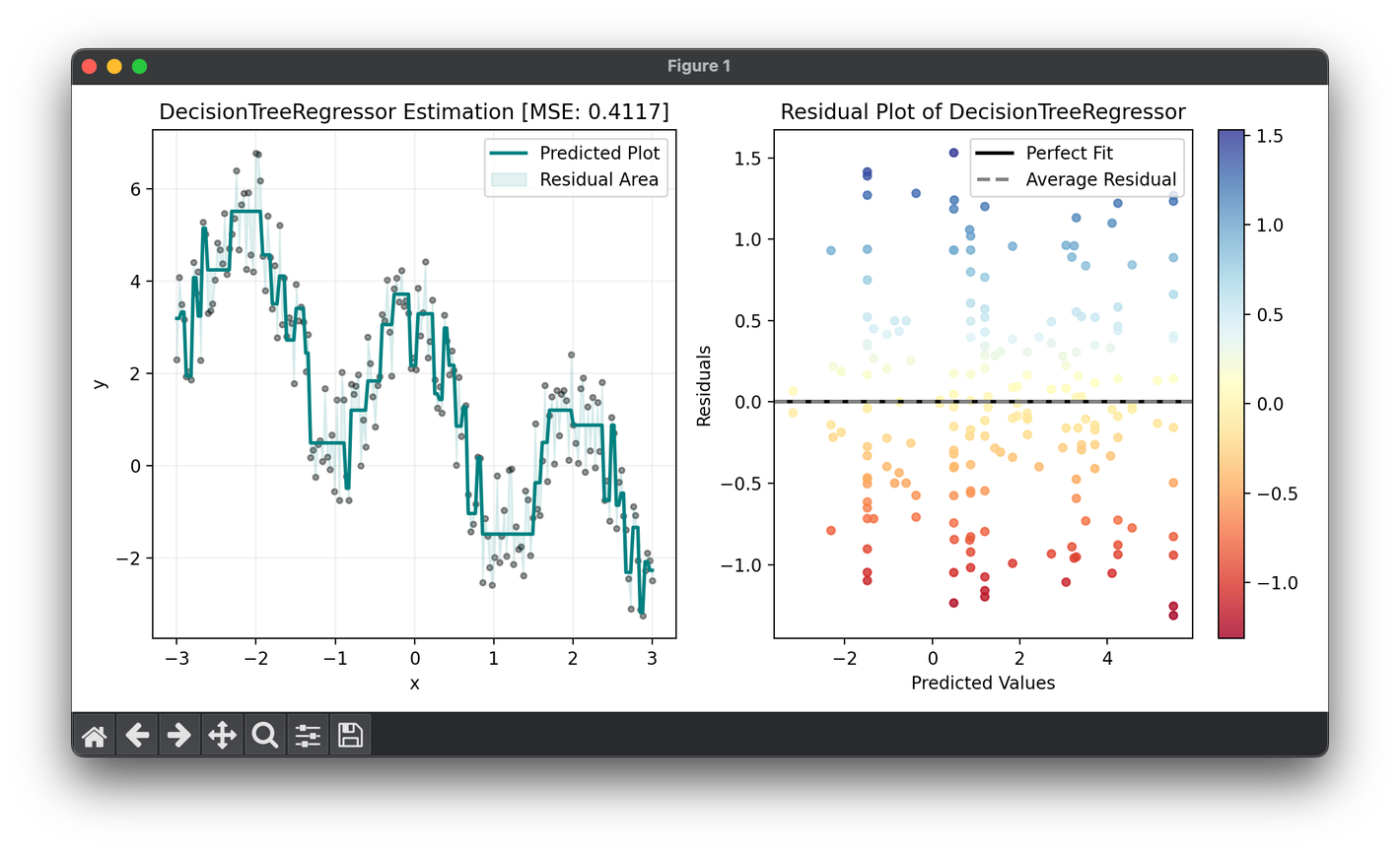
Examples

from luma.regressor.tree import DecisionTreeRegressor
from luma.visual.evaluation import ResidualPlot

import matplotlib.pyplot as plt
import numpy as np

np.random.seed(42)

X = np.linspace(-3, 3, 200).reshape(-1, 1)
y = (2 * np.cos(3 * X) - X).flatten() + 3 * np.random.rand(200)

tree = DecisionTreeRegressor(max_depth=6)
tree.fit(X, y)
y_pred = tree.predict(X)

fig = plt.figure(figsize=(10, 5))
ax1 = fig.add_subplot(1, 2, 1)
ax2 = fig.add_subplot(1, 2, 2)

ax1.scatter(X, y, s=10, c="black", alpha=0.4)
ax1.plot(X, y_pred, lw=2, c="teal", label="Predicted Plot")
ax1.fill_between(
    X.flatten(), y_pred, y, color="teal", alpha=0.1, label="Residual Area"
)
ax1.set_xlabel("x")
ax1.set_ylabel("y")
ax1.set_title(f"{type(tree).__name__} Estimation [MSE: {tree.score(X, y):.4f}]")
ax1.legend()
ax1.grid(alpha=0.2)

res = ResidualPlot(tree, X, y)
res.plot(ax=ax2, show=True)

Applications

• Real Estate Pricing: Predicting house prices based on features like location, size, and amenities.
• Energy Consumption: Forecasting energy use in buildings or areas based on historical usage patterns and weather data.
• Stock Price Prediction: Estimating future stock prices based on various economic indicators.

Strengths and Limitations

Strengths

• Interpretability: Decision trees are easy to understand and interpret, making them useful for gaining insights into the data.
• Non-linearity: Capable of capturing non-linear relationships without the need for data transformation.
• No need for feature scaling: Unlike many other regression methods, decision trees do not require feature scaling to perform well.

Limitations

• Overfitting: Without proper constraints, trees can grow very deep and complex, leading to overfitting.
• Instability: Small changes in the data can lead to significantly different tree structures.
• Predictive Performance: Generally, decision tree regression does not have the same level of predictive accuracy as some other regression methods, especially for tasks with complex relationships.

Advanced Topics

Ensemble Methods

Improving decision tree regression performance often involves using ensemble methods, such as Random Forests and Gradient Boosted Trees. These methods build multiple trees and aggregate their predictions to improve accuracy and robustness.

Pruning

Pruning is a technique used to reduce the size of

a decision tree by removing parts of the tree that do not provide additional power to classify instances. This can help improve the model's generalizability and reduce overfitting.

References

1. L. Breiman, J. Friedman, R. Olshen, and C. Stone. "Classification and Regression Trees". Wadsworth, 1984.
2. T. Hastie, R. Tibshirani, and J. Friedman. "The Elements of Statistical Learning: Data Mining, Inference, and Prediction". Springer Series in Statistics, 2009.
3. S. Raschka. "Python Machine Learning". Packt Publishing, 2015.