Kernel Support Vector Regression (Kernel SVR)

Introduction

Kernel Support Vector Regression (Kernel SVR) is an advanced machine learning algorithm that extends the concept of Support Vector Regression (SVR) by employing kernel functions. This technique allows for modeling complex, non-linear relationships between the dependent and independent variables in a dataset. Originally developed from the principles of Support Vector Machines (SVM) for classification, SVR and its kernelized version have been successfully applied in various regression tasks where precision and robustness against outliers are crucial.

Background and Theory

Support Vector Regression (SVR)

Support Vector Regression is a type of regression analysis that aims to find the best fitting line (in two dimensions) or hyperplane (in higher dimensions) that has the maximum number of points within a certain threshold (epsilon). The concept revolves around the idea of minimizing error, ensuring that predictions fall within a specified epsilon margin, while simultaneously trying to keep the model as simple and generalized as possible.

The Kernel Trick

The kernel trick is a mathematical technique that enables linear classifiers to operate in a transformed feature space, allowing them to solve non-linear problems without explicitly mapping data to a higher-dimensional space. This is achieved by using a kernel function to compute the dot product of the vectors in this higher-dimensional space. Common kernel functions include:

• Linear Kernel: $K(\mathbf{x}, \mathbf{x}') = \mathbf{x}^\top \mathbf{x}'$
• Polynomial Kernel: $K(\mathbf{x}, \mathbf{x}') = (\gamma\mathbf{x}^\top \mathbf{x}' + r)^d$, where $\gamma$, $r$, and $d$ are parameters.
• Radial Basis Function (RBF) Kernel: $K(\mathbf{x}, \mathbf{x}') = \exp(-\gamma \|\mathbf{x} - \mathbf{x}'\|^2)$, where $\gamma$ is a parameter.
• Sigmoid Kernel: $K(\mathbf{x}, \mathbf{x}') = \tanh(\gamma\mathbf{x}^\top \mathbf{x}' + r)$

Kernel SVR Formulation

Kernel SVR uses the kernel trick to map the input features into a high-dimensional space where a linear regression surface is sought. The objective function of Kernel SVR is to minimize:

Subject to:

Where:

• $\mathbf{w}$ is the weight vector in the transformed feature space.
• $C$ is the regularization parameter.
• $\xi_i$ and $\xi_i^*$ are slack variables representing the distance from the actual values to the respective margins for points outside the epsilon margin.
• $\phi$ is the function used to transform data into a higher-dimensional space.
• $b$ is the bias.
• $\epsilon$ represents the width of the margin.

Through the dual formulation and the use of Lagrange multipliers, the kernelized version eliminates the need to explicitly know $\phi$, instead requiring only the computation of the kernel function $K(\mathbf{x}, \mathbf{x}')$.

Implementation

Parameters

• C: float, default = 1.0
  Regularization parameter
  
• deg: int, default = 2
  Polynomial degree
  
• gamma: float, default = 1.0
  Shape parameter of Gaussian curve for RBF kernel
  
• coef: float, default = 1.0
  Coefficient for ‘poly’ and ‘sigmoid’ kernel
  
• learning_rate: float, default = 0.001
  Step-size for gradient descent update
  
• max_iter: int, default = 1000
  Number of iteration
  
• kernel: FuncType, default = ‘rbf’
  Type of kernel
  

Examples

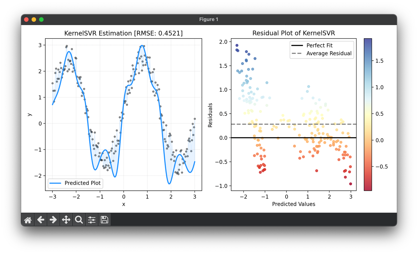
from luma.regressor.svm import KernelSVR
from luma.visual.evaluation import ResidualPlot

import matplotlib.pyplot as plt
import numpy as np

n_samples = 200

X = np.linspace(-3, 3, n_samples).reshape(-1, 1)
y = (2 * np.sin(2 * X) + np.random.rand(n_samples, 1)).flatten()

reg = KernelSVR(learning_rate=0.1, gamma=10, kernel="rbf")
reg.fit(X, y)
y_pred = reg.predict(X)
score = reg.score(X, y)

fig = plt.figure(figsize=(10, 5))
ax1 = fig.add_subplot(1, 2, 1)
ax2 = fig.add_subplot(1, 2, 2)

ax1.scatter(X, y, s=10, c="black", alpha=0.4)
ax1.plot(X, y_pred, lw=2, c="dodgerblue", label="Predicted Plot")
ax1.fill_between(X.flatten(), y, y_pred, color="dodgerblue", alpha=0.1)
ax1.set_xlabel("x")
ax1.set_ylabel("y")
ax1.set_title(f"{type(reg).__name__} Estimation [RMSE: {score:.4f}]")
ax1.legend()
ax1.grid(alpha=0.2)

res = ResidualPlot(reg, X, y)
res.plot(ax=ax2, show=True)

Applications

Kernel SVR has been extensively applied in fields requiring the prediction of continuous variables, especially where the relationship between the dependent and independent variables is nonlinear. Common applications include:

• Finance: Predicting stock prices and market trends.
• Energy: Forecasting demand and supply in power systems.
• Environment: Modeling climate data and pollution levels.
• Healthcare: Predicting disease progression and patient outcomes.

Strengths and Limitations

Strengths

• Flexibility: Can model non-linear relationships effectively.
• Robustness: Less sensitive to outliers than traditional regression models.
• Generalization: Tends to perform well on unseen data due to its regularization and margin properties.

Limitations

• Parameter Sensitivity: The performance heavily depends on the choice of the kernel function and its parameters, as well as the regularization parameter $C$.
• Computational Complexity: Can be computationally intensive, especially with large datasets.
• Interpretability: The transformation into a high-dimensional space can make the model difficult to interpret compared to simpler regression models.

Advanced Topics

• Hyperparameter Tuning: Techniques for optimizing the choice of kernel, $C$, $\epsilon$, and kernel-specific parameters.
• Feature Engineering: Preprocessing and feature selection methods that can enhance the performance of Kernel SVR.
• Ensemble Methods: Combining multiple Kernel SVR models to improve prediction accuracy and robustness.

References

1. Vapnik, Vladimir. "The nature of statistical learning theory." Springer science & business media, 2013.
2. Drucker, Harris, et al. "Support vector regression machines." Advances in neural information processing systems, 1997.
3. Schölkopf, Bernhard, and Alexander J. Smola. "Learning with kernels: support vector machines, regularization, optimization, and beyond." MIT press, 2002.