Elastic Net Regression

Introduction

Elastic Net Regression is an advanced regularization technique that synergizes the regularization aspects of both Lasso (L1 regularization) and Ridge (L2 regularization) regression methods. It addresses the limitations and harnesses the strengths of both methods, making it particularly effective for datasets with high multicollinearity or when the number of predictors exceeds the number of observations. This document elaborates on Elastic Net Regression, focusing on sophisticated optimization strategies including gradient computations and soft-thresholding mechanisms.

Background and Theory

Linear Regression Fundamentals

Linear regression models the relationship between a dependent variable $Y$ and a set of independent variables $\{X_1, X_2, \ldots, X_p\}$ as:

where $\beta_0, \beta_1, \ldots, \beta_p$ are coefficients, and $\epsilon$ represents the error term.

Regularization: Bridging Lasso and Ridge

Lasso regression applies an L1 penalty leading to sparse solutions, where some coefficients can become exactly zero, aiding in feature selection. Ridge regression employs an L2 penalty, which shrinks coefficients but does not zero them out, helping to deal with multicollinearity. Elastic Net combines these approaches, incorporating both L1 and L2 penalties into its cost function.

Elastic Net Regression Overview

The Elastic Net cost function is expressed as:

where $n$ is the number of observations, $\lambda$ is the overall strength of the regularization, and $\alpha$ blends the L1 and L2 penalties, with values ranging from 0 (ridge) to 1 (Lasso).

Mathematical Formulation

Objective Function

The Elastic Net objective combines the Ridge and Lasso penalties:

This formulation allows Elastic Net to inherit the feature selection ability of Lasso and the group effect of Ridge, suitable for correlated predictors.

Coordinate Descent

The non-differentiability of the L1 penalty at zero complicates the optimization process. Coordinate descent emerges as a powerful method for solving the Elastic Net problem, iteratively optimizing the loss function one coefficient at a time while holding others fixed.

Gradient Computation

For the Ridge part, the gradient with respect to $\beta_j$ can be derived and used in gradient descent steps. However, due to the absolute value in the Lasso penalty, direct gradient computation is not straightforward for the L1 component.

Soft-Thresholding for Lasso Component

Soft-thresholding is applied to handle the L1 penalty, a technique that emerges from the subgradient method for optimization. For each coefficient $\beta_j$, the soft-thresholding operator is applied as:

where $z_j$ is the partial residual obtained by excluding $\beta_j$, and $S_{\lambda \alpha}(\cdot)$ is the soft-thresholding function defined by:

This step essentially shrinks coefficients towards zero, with those falling below a certain threshold being set to zero, hence enforcing sparsity.

Implementation

Parameters

• alpha: float, default = 1.0
  Regularization strength
  
• l1_ratio: float, default = 0.5
  Balancing parameter between L1 and L2 regularization
  
• max_iter: int, default = 100
  Number of iteration
  
• learning_rate: float, default = 0.01
  Step size of the gradient descent update
  

Examples

from luma.regressor.linear import ElasticNetRegressor
from luma.model_selection.search import GridSearchCV
from luma.metric.regression import MeanSquaredError
from luma.visual.evaluation import ResidualPlot

import matplotlib.pyplot as plt
import numpy as np

X = np.linspace(1, 5, 100).reshape(-1, 1)
y = np.log(X).flatten() + 0.2 * np.random.randn(100)

param_grid = {"alpha": np.logspace(-3, 3, 5),
              "learning_rate": np.logspace(-3, -1, 5),
              "l1_ratio": np.linspace(0, 1, 5)}

grid = GridSearchCV(estimator=ElasticNetRegressor(),
                    param_grid=param_grid,
                    cv=5,
                    metric=MeanSquaredError,
                    maximize=False,
                    refit=True,
                    shuffle=True,
                    random_state=42)

grid.fit(X, y)
print(grid.best_params, grid.best_score)
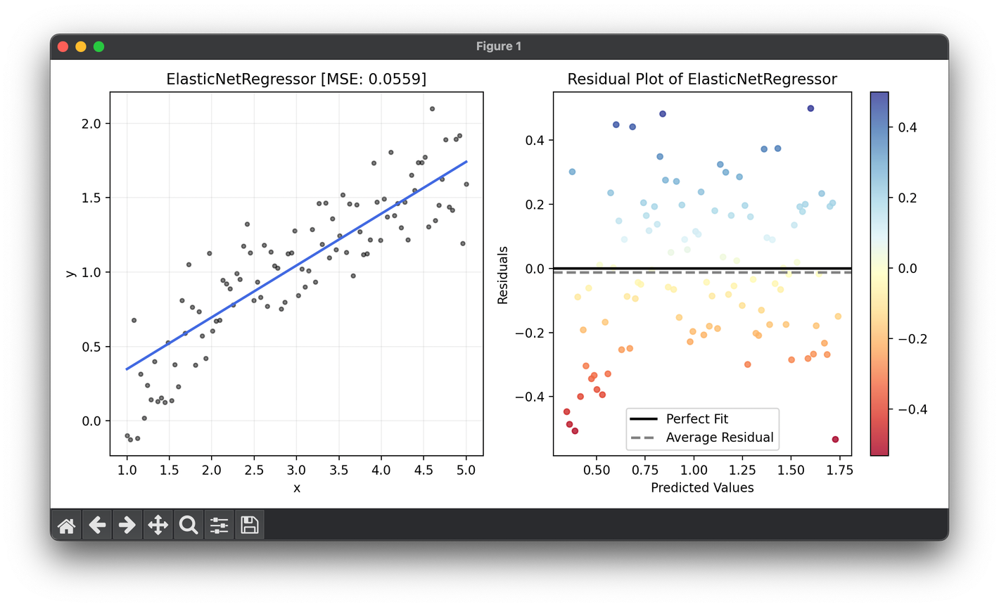
reg = grid.best_model

fig = plt.figure(figsize=(10, 5))
ax1 = fig.add_subplot(1, 2, 1)
ax2 = fig.add_subplot(1, 2, 2)

ax1.scatter(X, y, s=10, c="black", alpha=0.5, label=r"y=x+\epsilon")
ax1.plot(X, reg.predict(X), lw=2, c="royalblue")
ax1.set_xlabel("x")
ax1.set_ylabel("y")
ax1.set_title(f"{type(reg).__name__} [MSE: {reg.score(X, y):.4f}]")
ax1.grid(alpha=0.2)

res = ResidualPlot(reg, X, y)
res.plot(ax=ax2, show=True)

Applications

Elastic Net is versatile, finding applications in various domains such as:

• Predictive Modeling: Where both feature selection and regularization are critical.
• Bioinformatics: For gene expression analysis where predictors are numerous and highly correlated.
• Finance: In constructing predictive models for stock prices, where it's essential to deal with multicollinearity among economic indicators.

Strengths and Limitations

Strengths

• Feature Selection and Group Effect: Elastic Net is capable of selecting variables and handling correlated data efficiently.
• Flexibility: The blend parameter $\alpha$ provides flexibility, allowing Elastic Net to adjust between Lasso and Ridge effects.

Limitations

• Parameter Selection: The necessity to tune multiple parameters ($\lambda$ and $\alpha$) can make the optimization process challenging.
• Computational Demand: The optimization process, particularly coordinate descent with soft-thresholding, can be computationally intensive.

Advanced Topics

Model Tuning and Selection

Model performance critically depends on the choice of $\lambda$ and $\alpha$. Techniques such as cross-validation are essential for identifying optimal parameter values.

Scaling Before Regularization

Standardizing predictors before applying Elastic Net is crucial due to the penalty on the size of coefficients, ensuring that regularization is uniformly applied.

References

1. Zou, Hui, and Trevor Hastie. "Regularization and variable selection via the elastic net." Journal of the Royal Statistical Society: Series B (Statistical Methodology) 67.2 (2005): 301-320.
2. Friedman, Jerome, Trevor Hastie, and Rob Tibshirani. "Regularization Paths for Generalized Linear Models via Coordinate Descent." Journal of Statistical Software 33.1 (2010).