Linear Regression

Introduction

Linear regression is a foundational statistical method used to model the relationship between a dependent variable and one or more independent variables. The objective is to find a linear function that best predicts the dependent variable from the independent variables. This document focuses on linear regression using Ordinary Least Squares (OLS) for parameter estimation, providing a thorough explanation of the OLS process, including its mathematical foundations, assumptions, and implications.

Theoretical Framework

Linear Regression Model

The general form of a linear regression model is:

where:

• $Y$ is the dependent variable.
• $X_1, X_2, \ldots X_p$ are the independent variables.
• $\beta_0, \beta_1, \ldots, \beta_p$ are the coefficients of the model.
• $\epsilon$ is the error term, representing unexplained variation in $Y$.

Objective of OLS

The primary goal of OLS is to estimate the coefficients ($\beta$) of the linear regression model in a way that minimizes the sum of the squared differences between the observed values and the values predicted by the model. This is known as minimizing the residual sum of squares (RSS).

Mathematical Formulation

OLS Estimation

The OLS estimates are obtained by minimizing the RSS:

where $\hat{y}_i$ is the predicted value for the $i$-th observation and $\hat{\beta}_0, \hat{\beta}_1, \ldots, \hat{\beta}_p$ are the OLS estimates of the coefficients.

Solving for Coefficients

To find the values of $\beta$ that minimize the RSS, we set the partial derivatives of the RSS with respect to each coefficient equal to zero. This yields a set of normal equations, which can be solved to get the OLS estimates:

In matrix notation, the solution can be compactly written as:

where $X$ is the matrix of input features (with each row representing an observation and each column a feature), and $Y$ is the vector of observed values of the dependent variable.

Implementation

Parameters

No parameters.

Examples

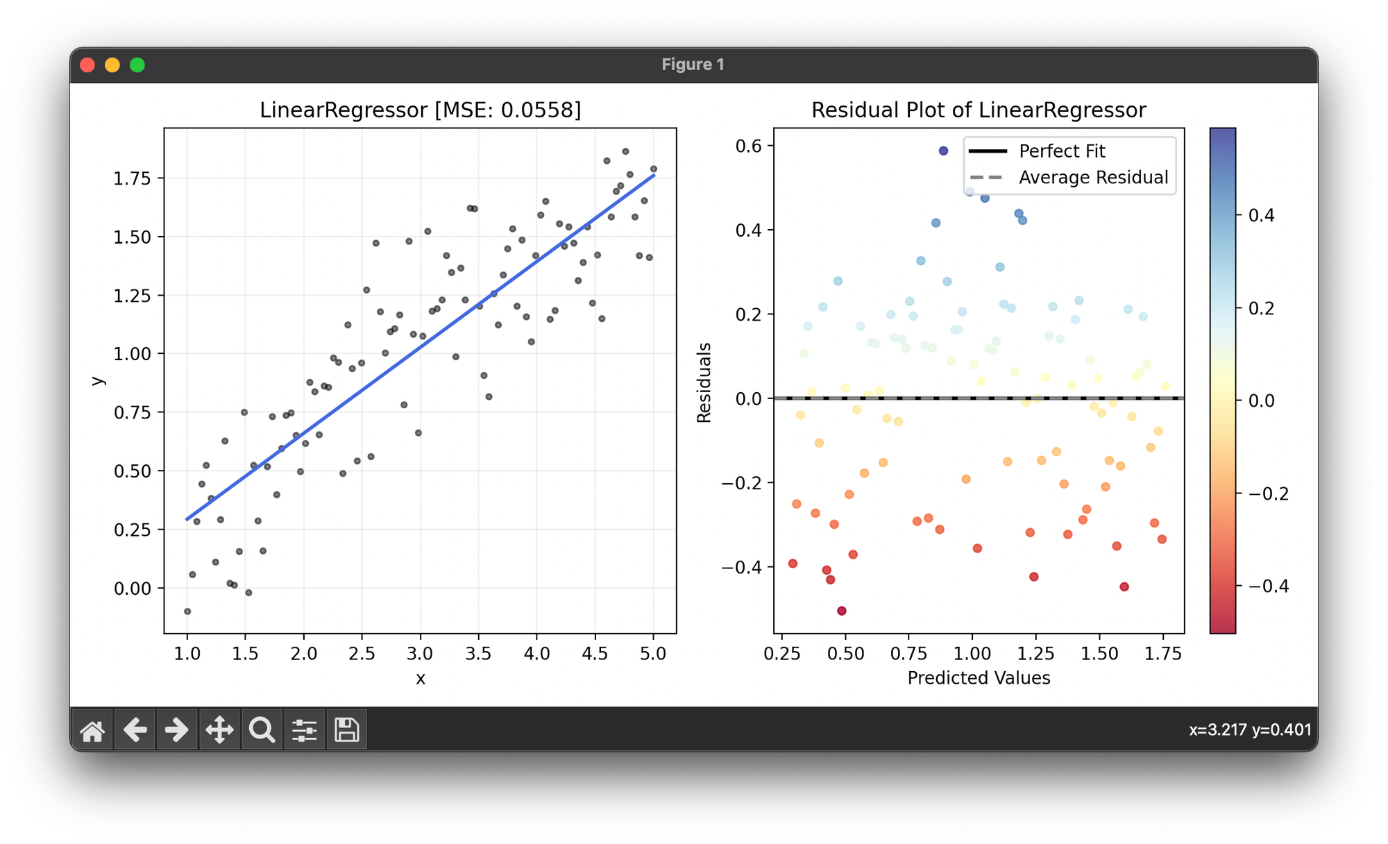
from luma.regressor.linear import LinearRegressor
from luma.visual.evaluation import ResidualPlot

import matplotlib.pyplot as plt
import numpy as np

X = np.linspace(1, 5, 100).reshape(-1, 1)
y = np.log(X).flatten() + 0.2 * np.random.randn(100)

reg = LinearRegressor()
reg.fit(X, y)

fig = plt.figure(figsize=(10, 5))
ax1 = fig.add_subplot(1, 2, 1)
ax2 = fig.add_subplot(1, 2, 2)

ax1.scatter(X, y, s=10, c="black", alpha=0.5, label=r"y=x+\epsilon")
ax1.plot(X, reg.predict(X), lw=2, c="royalblue")
ax1.set_xlabel("x")
ax1.set_ylabel("y")
ax1.set_title(f"{type(reg).__name__} [MSE: {reg.score(X, y):.4f}]")
ax1.grid(alpha=0.2)

res = ResidualPlot(reg, X, y)
res.plot(ax=ax2, show=True)

Assumptions of OLS

For OLS estimates to be considered the best, linear, unbiased estimates (BLUE), the following assumptions must hold:

1. Linearity: The relationship between the dependent and independent variables is linear.
2. Independence: Observations are independent of each other.
3. Homoscedasticity: The variance of error terms is constant across all levels of the independent variables.
4. No Multicollinearity: Independent variables are not too highly correlated.
5. Normality of Errors: The error terms are normally distributed (this assumption is more important for inference than for estimation).

Implications of OLS

• Efficiency: When the assumptions of OLS are met, it provides the most efficient (lowest variance) estimates of the regression coefficients.
• Interpretability: OLS regression coefficients can be directly interpreted in terms of the change in the dependent variable for a one-unit change in an independent variable, holding all other variables constant.

Applications and Limitations

Applications

Linear regression is widely used across various fields for predictive modeling, including economics, finance, biology, and social sciences.

Limitations

• Outliers: OLS is sensitive to outliers, which can significantly impact the regression line.
• Non-linearity: It cannot model nonlinear relationships without transformation of variables.
• Homoscedasticity Violation: Heteroscedasticity can lead to inefficient estimates and incorrect standard errors.

Conclusion

OLS is a cornerstone of linear regression analysis, providing a simple yet powerful method for estimating the relationship between variables. Understanding the assumptions and limitations of OLS is crucial for correctly applying the method and interpreting its results. By adhering to these principles, analysts can leverage linear regression to uncover meaningful insights from data across a multitude of domains.