Support Vector Regression (SVR)

Introduction

Support Vector Regression (SVR) extends the principles of Support Vector Machines (SVMs) from classification to regression problems. Developed from the foundation laid by Vapnik and others in the Support Vector Machine framework, SVR provides a unique approach to regression by focusing on fitting the error within a certain threshold and is particularly known for its robustness and effectiveness in high-dimensional spaces.

Background and Theory

SVR is grounded in the concept of SVM, which constructs a hyperplane or set of hyperplanes in a high-dimensional space to separate different classes. For regression, SVR attempts to find a function that has at most $\epsilon$ deviation from the actually obtained targets for all the training data, and at the same time, is as flat as possible.

Mathematical Foundations

In SVR, the input data $\mathbf{x}_i$ is mapped onto a high-dimensional feature space using a kernel function, and then a linear model is built in this feature space:

where $\mathbf{w}$ is the weight vector, $\phi(\mathbf{x})$ is the high-dimensional feature space mapped from the input vector $\mathbf{x}$, and $b$ is the bias. The goal is to minimize:

subject to the constraints:

Here, $\xi_i$ and $\xi_i^*$ are slack variables that measure the degree of violation of the $\epsilon$-insensitive loss, $C$ is the regularization parameter, and $\epsilon$ defines the width of the tube within which predictions are considered acceptable without penalty.

Procedural Steps

1. Kernel Selection: Choose an appropriate kernel function (linear, polynomial, radial basis function, sigmoid, etc.) that best suits the data distribution.
2. Parameter Tuning: Determine the values for $C$, $\epsilon$, and any parameters specific to the kernel (e.g., the degree of the polynomial kernel).
3. Training: Solve the optimization problem to find the optimal $\mathbf{w}$ and $b$ that minimize the regularized risk function.
4. Prediction: For a new input $\mathbf{x}$, predict the output using the learned function $f(\mathbf{x})$.

Mathematical Formulations

Dual Problem

The primal problem is often solved in its dual form to exploit kernel methods, leading to:

subject to:

Here, $\alpha_i$ and $\alpha_i^*$ are Lagrange multipliers, and $K(\mathbf{x}_i, \mathbf{x}_j) = \phi(\mathbf{x}_i)^T \phi(\mathbf{x}_j)$ is the kernel function.

Implementation

Parameters

• C: float, default = 1.0
  Regularization parameter
  
• epsilon: float, default = 0.1
  Epsilon-tube in the training loss function
  
• batch_size: int, default = 100
  Size of a single batch
  
• learning_rate: float, default = 0.001
  Step-size of gradient descent update
  
• max_iter: int, default = 1000
  Number of iteration
  

Examples

from luma.regressor.svm import SVR
from luma.model_selection.search import GridSearchCV
from luma.metric.regression import MeanSquaredError
from luma.visual.evaluation import ResidualPlot

import matplotlib.pyplot as plt
import numpy as np

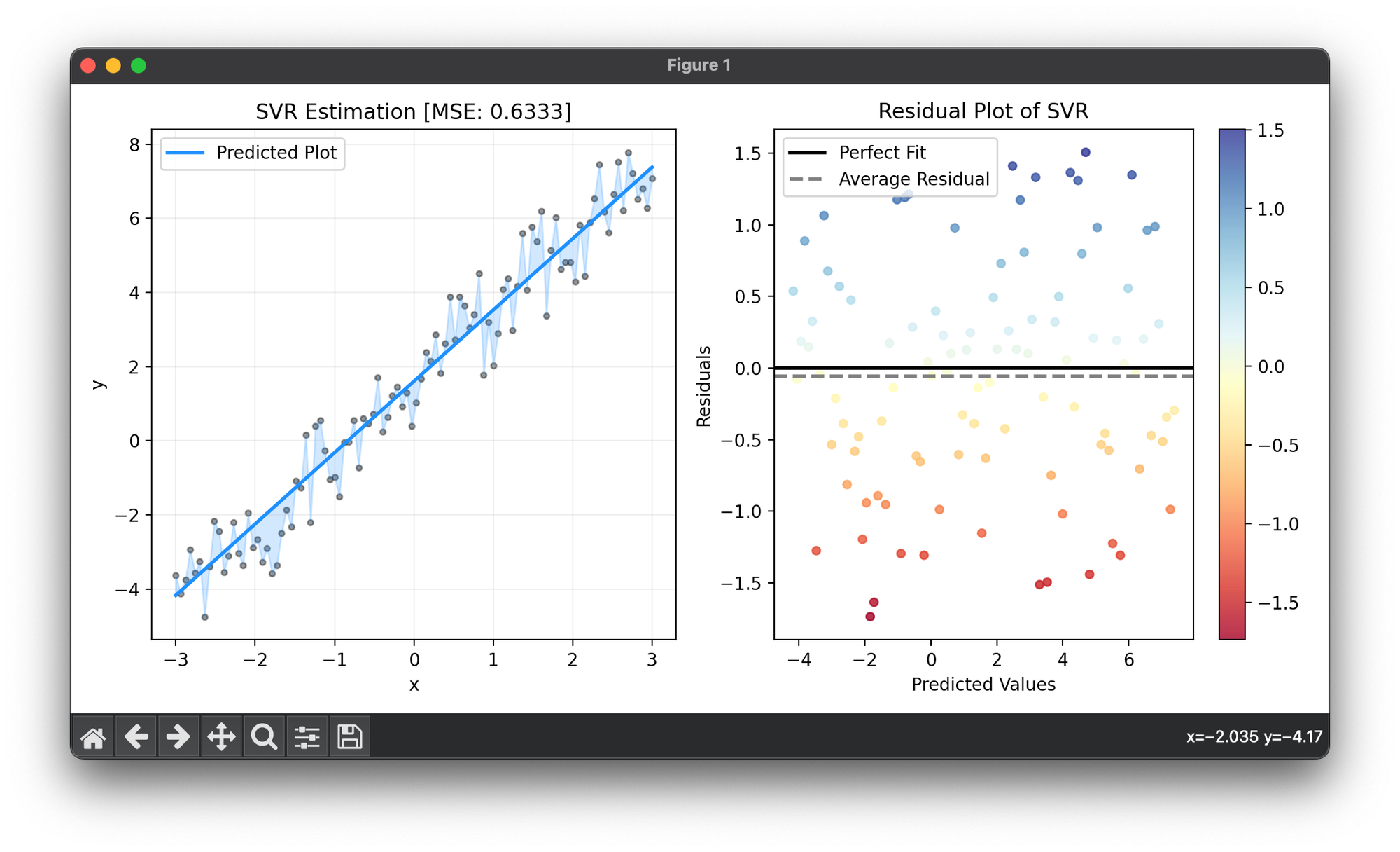
n_samples = 100

X = np.linspace(-3, 3, n_samples).reshape(-1, 1)
y = (2 * X + 3 * np.random.rand(n_samples, 1)).flatten()

param_grid = {"C": np.logspace(-3, 3, 5), 
              "learning_rate": np.logspace(-3, -1, 5)}

grid = GridSearchCV(estimator=SVR(),
                    param_grid=param_grid,
                    cv=5,
                    metric=MeanSquaredError,
                    maximize=False,
                    refit=True,
                    shuffle=True,
                    random_state=42,
                    verbose=True)
grid.fit(X, y)
print(grid.best_params, grid.best_score)
reg = grid.best_model
y_pred = reg.predict(X)
score = reg.score(X, y, metric=MeanSquaredError)

fig = plt.figure(figsize=(10, 5))
ax1 = fig.add_subplot(1, 2, 1)
ax2 = fig.add_subplot(1, 2, 2)

ax1.scatter(X, y, s=10, c="black", alpha=0.4)
ax1.plot(X, y_pred, lw=2, c="dodgerblue", label="Predicted Plot")
ax1.fill_between(X.flatten(), y, y_pred, color="dodgerblue", alpha=0.2)
ax1.set_xlabel("x")
ax1.set_ylabel("y")
ax1.set_title(f"{type(reg).__name__} Estimation [MSE: {score:.4f}]")
ax1.legend()
ax1.grid(alpha=0.2)

res = ResidualPlot(reg, X, y)
res.plot(ax=ax2, show=True)

Applications

• Finance: Predicting stock prices, risk management, and option pricing.
• Energy: Forecasting electricity demand and renewable energy output.
• Healthcare: Modeling disease progression and predicting patient outcomes.
• Environmental Science: Estimating air quality indices and climate modeling.

Strengths and Limitations

Strengths:

• Flexibility: The ability to model nonlinear relationships through kernel trick.
• Robustness: Effective in high-dimensional spaces and relatively immune to overfitting when properly regularized.
• Sparcity: Only support vectors contribute to the decision function, making the model efficient.

Limitations:

• Parameter Sensitivity: Choosing the right kernel and tuning parameters can be challenging.
• Scalability: Computational complexity increases significantly with the size of the dataset.

Advanced Topics

• Kernel Methods: Exploring different kernel functions to capture complex relationships in the data.
• Multi-output SVR: Extending SVR for scenarios where multiple outputs are predicted simultaneously.
• Deep SVR: Integrating SVR with deep learning architectures for enhanced feature representation and prediction accuracy.

References

1. Vapnik, Vladimir. "The nature of statistical learning theory." Springer Science & Business Media, 2013.
2. Smola, Alex J., and Bernhard Schölkopf. "A tutorial on support vector regression." Statistics and computing 14.3 (2004): 199-222.