Costa Rican Household Poverty Level Prediction - 3. Individual Level Variables

3. Individual Level Variables

• Individual level variable에는 2가지 종류가 있다

1. 참/거짓을 나타내는 Boolean값
2. 순서를 나타내는 값

ind = data[id_ + ind_bool + ind_ordered]
ind.shape

3.1 Redundant Individual Variables

• 필요 없는 변수들을 제거하기 위해 상관계수 절댓값이 0.95가 넘어가는 것만 남기도록 한다

# 상관계수 매트릭스 만들기
corr_matrix = ind.corr()

upper = corr_matrix.where(np.triu(np.ones(corr_matrix.shape), k = 1).astype(np.bool))

to_drop = [column for column in upper.columns if any(abs(upper[column]) > 0.95)]

to_drop

• female 상관계수가 굉장히 높으므로 그 반대인 male 컬럼을 버린다

ind = ind.drop(columns = 'male')

3.1.1 Creating Ordinal Variables

• instlevel1 : 교육 X ~ instlevel9 : 대학원 졸업 까지의 교육 수준을 나타내는 컬럼 생성

ind[[c for c in ind if c.startswith('instl')]].head()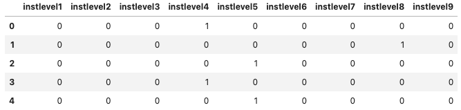

ind['inst'] = np.argmax(np.array(ind[[c for c in ind if c.startswith('instl')]]), axis = 1)
plot_categoricals('inst', 'Target', ind, annotate = False)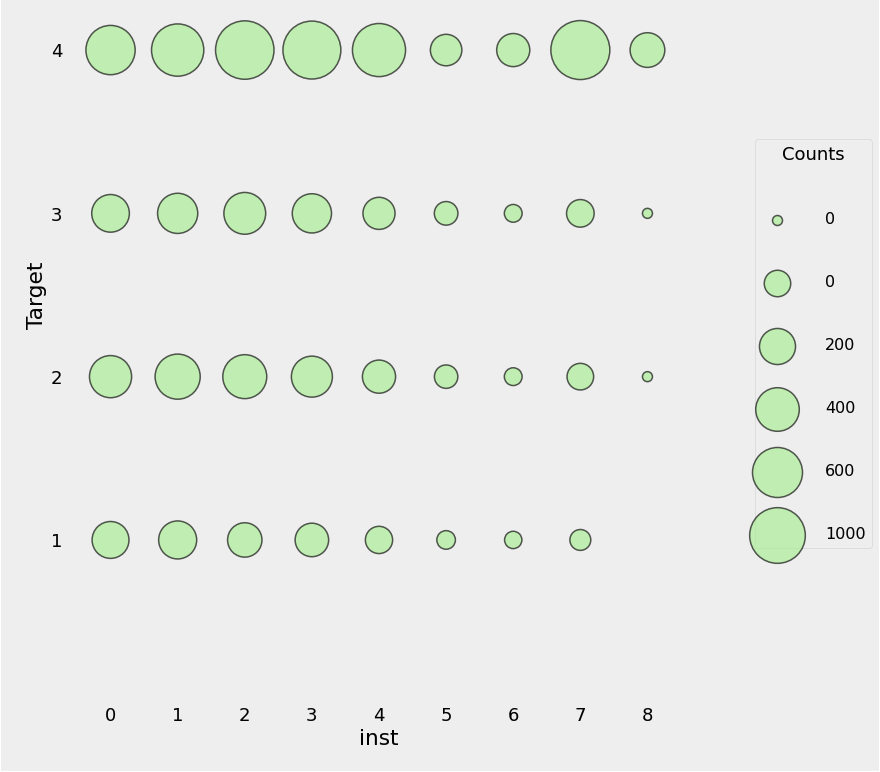

• 위의 결과를 보아, 교육수준이 높을수록 가난지수가 낮은 것을 확인할 수 있다

plt.figure(figsize = (10. 8))
sns.violinplot(x = 'Target', y = 'inst', data = ind)
plt.title('Education Distribution by Target')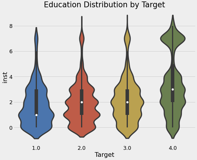

3.1.2 Feature Construction

• 기존에 존재하는 데이터로 새로운 데이터 만들기

ind['escolari/age'] = ind['escolari'] / ind['age']

plt.figure(figsize = (10, 8))
sns.violinplot('Target', 'escolari.age', data = ind)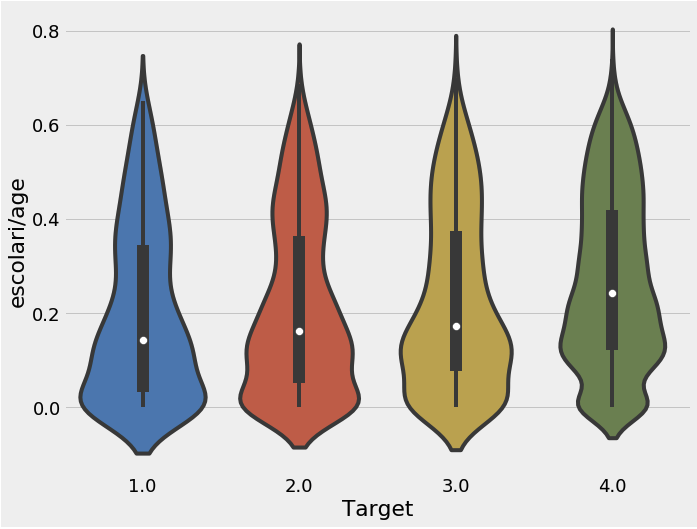

ind['inst/age'] = ind['inst'] / ind['age']
ind['tech'] = ind['v18q'] + ind['mobilephone']
ind['tech'].describe()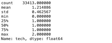

3.2 Feature Engineering through Aggregations

range_ = lambda x: x.max() - x.min()
range_.__name__ = 'range_'

ind_agg = ind.drop(columns = 'Target').groupby('idhogar').agg(['min','max','sum','count','std',range_])
ind_agg.head()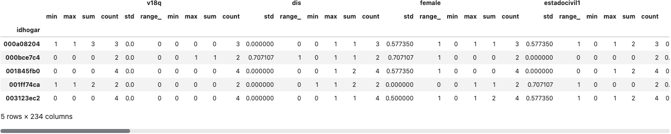

• 컬럼 이름 재정의

new_col = []
for c in ind_agg.columns.levels[0]:
    for stat in ind_agg.columns.levels[1]:
        new_col.append(f'{c}-{stat}')
        
ind_agg.columns = new_col
ind_agg.head()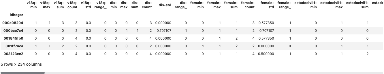

ind_agg.iloc[:, [0, 1, 2, 3, 6, 7, 8, 9]].head()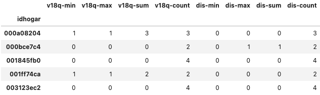

3.2.1 Feature Selection

corr_matrix = ind_agg.corr()

upper = corr_matrix.where(np.triu(np.ones(corr_matrix.shape), k = 1).astype(np.bool))

to_drop = [column for column in upper.columns if any(abs(upper[column]) > 0.95)]

print(f'There are {len(to_drop)} correlated columns to remove')

ind_agg = ind_agg.drop(columns = to_drop)
ind_feats = list(ind_agg.columns)

final = heads.merge(ind_agg, on = 'idhogar', how = 'left')

print('Final features shape: ', final.shape)

final.head()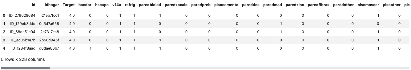

3.2.2 Final Data Exploration

corrs = final.corr()['Target']

corrs.sort_values().dropna().tail()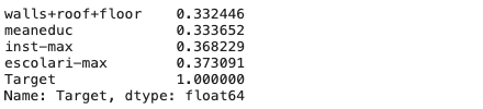

plot_categoricals('escolari-max', 'Target', final, annotate=False);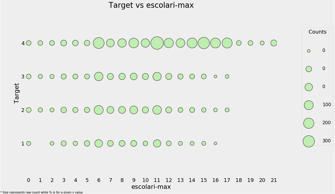

plt.figure(figsize = (10, 6))
sns.violinplot(x = 'Target', y = 'escolari-max', data = final)
plt.title('Max Schooling by Target')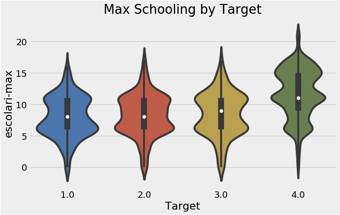

plt.figure(figsize = (10, 6))
sns.boxplot(x = 'Target', y = 'escolari-max', data = final)
plt.title('Max Schooling by Target')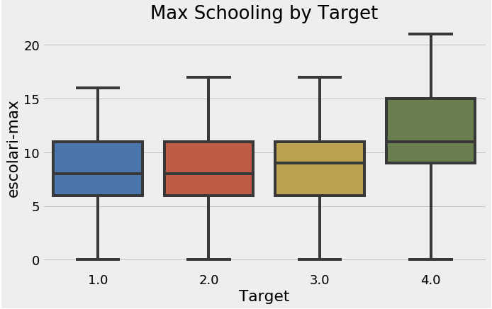

plt.figure(figsize = (10, 6))
sns.boxplot(x = 'Target', y = 'overcrowding', data = final)
plt.xticks([0, 1, 2, 3], poverty_mapping.values())
plt.title('Overcrowding by Target')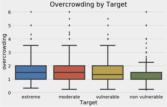

head_gender = ind.loc[ind['parentesco1'] == 1, ['idhogar', 'female']]
final = final.merge(head_gender, on = 'idhogar', how = 'left').rename(columns = {'female': 'female-head'})

final.groupby('female-head')['Target'].value_counts(normalize=True)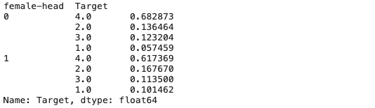

sns.violinplot(x = 'female-head', y = 'Target', data = final);
plt.title('Target by Female Head of Household');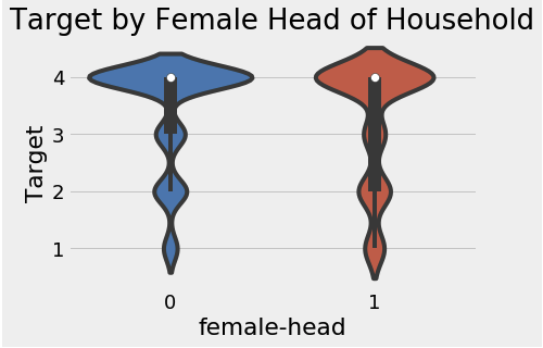

plt.figure(figsize = (8, 8))
sns.boxplot(x = 'Target', y = 'meaneduc', hue = 'female-head', data = final);
plt.title('Average Education by Target and Female Head of Household', size = 16);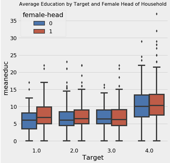

final.groupby('female-head')['meaneduc'].agg(['mean', 'count'])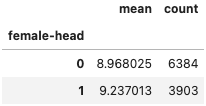

• 대체적으로 여성이 가장인 경우 더 높은 교육 수준을 가지는 것으로 보였다
• 그러나 동시에