Intro
얼마 전 캐글에서 구글 Jigsaw/Conversation AI팀에 의해 'Jigsaw Unintended Bias in Toxicity Classification'라는 주제로 competition이 개최되어 호기심에 도전해보았다.

Jigsaw라는 곳을 처음 들어봤는데 알아보니 구글의 자회사로 온라인 상의 욕설이나 선동적, 폭력적 대화를 잡아내는 기술을 연구하는 곳이었고,
Description상에 의한 이 Competition의 주요문제는 다음과 같았다.
현재 Jigsaw의 Conversation AI팀은 Perspective라는 제품을 통해 온라인 상의 악성 대화(위협, 외설, 모욕 등)를 잡아내고 있는데, 모델을 좀 더 정교하게 하여 낮은 에러율의 다양한 악성 대화를 잡아내는 모델을 만드는 것.
데이터의 경우 train데이터와 test데이터를 따로 제공하며, train 데이터의 경우 180만건 정도 되는데 텍스트 데이터 위주로 되어있다보니 사이즈가 상당히 컸다.
해당 competition의 결과 제출은 Kernels에 의해서만 가능한데, 데이터 사이즈가 크다보니 모델에 의한 학습도 굉장히 오래걸리고 kaggle내에서도 kernel 학습시간에 제한을 두기 때문에 모델을 정교하게 학습시키는 것이 쉽지 않았다.
코드 작성은 Jupyter notebook을 이용하였으며, 아래 작성된 코드는 ipynb파일을 markdown으로 변환하여 업로드하였다.
Import Library
import os
import numpy as np
import pandas as pd
import matplotlib.pyplot as plt
from collections import Counter
import nltk
nltk.download('stopwords')
nltk.download('punkt')
from nltk.corpus import stopwords
from nltk.tokenize import word_tokenize
stop_words = set(stopwords.words('english'))
import tensorflow as tf
from sklearn.metrics import roc_auc_score
from keras import models, layers, Model
from keras.preprocessing import text, sequence
from keras.callbacks import EarlyStopping, ModelCheckpoint, ReduceLROnPlateau
import os
print(os.listdir("./input"))
['test.csv', 'train.csv']1. Load Data
- 데이터는 train 데이터가 180만건, test 데이터가 9만7천건 정도로 이루어져 있다.
- train 데이터는 id, target, comment_text를 포함하여 총 45개의 칼럼으로 이루어져 있지만, test 데이터의 경우 id, target, comment_text 총 3개의 칼럼으로만 이루어져 있다.
## load data
train_data = pd.read_csv('./input/train.csv')
test_data = pd.read_csv('./input/test.csv')
print(train_data.shape)
print(test_data.shape)
(1804874, 45)
(97320, 2)train_data.head()| id | target | comment_text | severe_toxicity | obscene | identity_attack | insult | threat | asian | atheist | ... | article_id | rating | funny | wow | sad | likes | disagree | sexual_explicit | identity_annotator_count | toxicity_annotator_count | |
|---|---|---|---|---|---|---|---|---|---|---|---|---|---|---|---|---|---|---|---|---|---|
| 0 | 59848 | 0.000000 | This is so cool. It's like, 'would you want yo... | 0.000000 | 0.0 | 0.000000 | 0.00000 | 0.0 | NaN | NaN | ... | 2006 | rejected | 0 | 0 | 0 | 0 | 0 | 0.0 | 0 | 4 |
| 1 | 59849 | 0.000000 | Thank you!! This would make my life a lot less... | 0.000000 | 0.0 | 0.000000 | 0.00000 | 0.0 | NaN | NaN | ... | 2006 | rejected | 0 | 0 | 0 | 0 | 0 | 0.0 | 0 | 4 |
| 2 | 59852 | 0.000000 | This is such an urgent design problem; kudos t... | 0.000000 | 0.0 | 0.000000 | 0.00000 | 0.0 | NaN | NaN | ... | 2006 | rejected | 0 | 0 | 0 | 0 | 0 | 0.0 | 0 | 4 |
| 3 | 59855 | 0.000000 | Is this something I'll be able to install on m... | 0.000000 | 0.0 | 0.000000 | 0.00000 | 0.0 | NaN | NaN | ... | 2006 | rejected | 0 | 0 | 0 | 0 | 0 | 0.0 | 0 | 4 |
| 4 | 59856 | 0.893617 | haha you guys are a bunch of losers. | 0.021277 | 0.0 | 0.021277 | 0.87234 | 0.0 | 0.0 | 0.0 | ... | 2006 | rejected | 0 | 0 | 0 | 1 | 0 | 0.0 | 4 | 47 |
5 rows × 45 columns
2. Set index & target label
- 다른 커널을 보니 train 데이터의 다양한 칼럼을 활용하는 것 같던데 여기선 텍스트 데이터와 타겟 값만을 이용하여 학습 및 예측을 수행하였다.
- id 값은 index로 지정해두었으며, target값의 경우 Data Description의 설명에 따라 0.5이상은 positive 0.5미만은 negative 라벨로 분류하였다.
train_df = train_data[['id','comment_text','target']]
test_df = test_data.copy()

# set index
train_df.set_index('id', inplace=True)
test_df.set_index('id', inplace=True)

# y_label
train_y_label = np.where(train_df['target'] >= 0.5, 1, 0) # Label 1 >= 0.5 / Label 0 < 0.5
train_df.drop(['target'], axis=1, inplace=True)
# ratio by Class
Counter(train_y_label)Counter({0: 1660540, 1: 144334})3. View text data
- comment_text 칼럼을 출력해보면 아래와 같이 다양한 주제의 대화 내용을 확인할 수 있다.
train_data['comment_text'].head(20)0 This is so cool. It's like, 'would you want yo...
1 Thank you!! This would make my life a lot less...
2 This is such an urgent design problem; kudos t...
3 Is this something I'll be able to install on m...
4 haha you guys are a bunch of losers.
5 ur a sh*tty comment.
6 hahahahahahahahhha suck it.
7 FFFFUUUUUUUUUUUUUUU
8 The ranchers seem motivated by mostly by greed...
9 It was a great show. Not a combo I'd of expect...
10 Wow, that sounds great.
11 This is a great story. Man. I wonder if the pe...
12 This seems like a step in the right direction.
13 It's ridiculous that these guys are being call...
14 This story gets more ridiculous by the hour! A...
15 I agree; I don't want to grant them the legiti...
16 Interesting. I'll be curious to see how this w...
17 Awesome! I love Civil Comments!
18 I'm glad you're working on this, and I look fo...
19 Angry trolls, misogynists and Racists", oh my....
Name: comment_text, dtype: object4. Remove Punctuation & Stopword
- 가장 기본적인 텍스트 전처리를 위하여 간단히 텍스트 내의 punctuation과 stopwords를 제거하는 함수를 정의하였다.
- 워낙 데이터가 커서 함수 호출 시 처리 속도가 오래 걸린다. 그래서 속도를 위해 list comprehension과 lambda로 처리하였는데 그래도 처리까지 시간이 꽤 걸렸다.
## Clean Punctuation & Stopwords
class clean_text:
	def __init__(self, text):
		self.text = text

	# Remove Punctuation
	def rm_punct(text):
		punct = set([p for p in "/-'?!.,#$%\'()*+-/:;<=>@[\\]^_`{|}~`" + '""“”’' + '∞θ÷α•à−β∅³π‘₹´°£€\×™√²—–&'])
		text = [t for t in text if t not in punct]

		return "".join(text)

	# Remove Stopwords
	def rm_stopwords(text):
		word_tokens = word_tokenize(text)
		result = [w for w in word_tokens if w not in stop_words]

		return " ".join(result)
# remove punctuation
train_df['comment_text'] = train_df['comment_text'].apply(lambda x: clean_text.rm_punct(x))
test_df['comment_text'] = test_df['comment_text'].apply(lambda x: clean_text.rm_punct(x))
# remove stopwords
X_train = train_df['comment_text'].apply(lambda x: clean_text.rm_stopwords(x))
X_test = test_df['comment_text'].apply(lambda x: clean_text.rm_stopwords(x))5. Tokenize
- 전처리된 데이터를 keras.Tokenizer를 이용하여 sequences 데이터로 변환한다.
- Tokenizer의 처리 순서는 아래와 같다.
-- Tokenizer 객체를 통해 데이터를 토큰화시킨 후 각 토큰에 고유 index를 부여하여 word index 생성
-- texts_to_sequences()를 통해 word index를 기반으로 시퀀스 데이터 생성
-- pad_sequences()를 통해 padding 추가
## tokenize
max_words = 100000
tokenizer = text.Tokenizer(num_words=max_words) # Tokenizer 객체생성
tokenizer.fit_on_texts(X_train)	# 토큰 별 word index 생성

# texts_to_sequences
sequences_text_train = tokenizer.texts_to_sequences(X_train)
sequences_text_test = tokenizer.texts_to_sequences(X_test)

print(sequences_text_train[:5])
[[21, 2188, 39, 6, 3, 32, 1115, 116, 48, 91, 277, 26, 138],
[323, 21, 3, 25, 107, 142, 144, 105, 7, 159, 125, 9, 28],
[21, 9494, 2834, 94, 4342, 340, 1102, 4913],
[241, 90, 384, 316, 5764, 1027, 164, 6388],
[5230, 586, 998, 2593]]texts_to_sequences()함수를 이용하면 토큰화 된 문자들이 위와 같이 고유 index 번호로 바뀐 채 sequnce 형태로 출력된다.
# add padding
max_len = max(len(l) for l in sequences_text_train)
pad_train = sequence.pad_sequences(sequences_text_train, maxlen=max_len)
pad_test = sequence.pad_sequences(sequences_text_test, maxlen=max_len)

print(pad_train[:5])
array([[ 0, 0, 0, ..., 277, 26, 138],
[ 0, 0, 0, ..., 125, 9, 28],
[ 0, 0, 0, ..., 340, 1102, 4913],
[ 0, 0, 0, ..., 1027, 164, 6388],
[ 0, 0, 0, ..., 586, 998, 2593]])max_len 값은 방금 위에서 sequence로 변환한 데이터 중 가장 많은 word 수를 가지는 데이터의 길이를 받은 것이고,
모든 데이터를 그 길이 만큼 맞춰주기 위하여 pad_seqences()함수를 통해 0값을 채워주게 된다.
6. Embedding + LSTM model
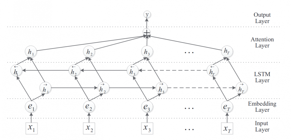
- 예측을 위해서 embedding 레이어와 lstm 레이어를 연결하여 딥러닝 모델을 구축하였다.
- Embedding 레이어는 텍스트 데이터의 단어 사이의 의미관계를 학습하는데 효과적이므로 텍스트 데이터 학습시 많이 사용되며,
- LSTM 모델은 양방향 LSTM(Bidirectional LSTM)으로 구축하여 시간적 의미와 상관없이 단어들 사이의 양방향적으로 의미 순서를 학습하도록 하였다.
def Embedding_CuDNNLSTM_model(max_words, max_len):
	sequence_input = layers.Input(shape=(None, ))
	x = layers.Embedding(max_words, 128, input_length=max_len)(sequence_input)
	x = layers.SpatialDropout1D(0.3)(x)
	x = layers.Bidirectional(layers.CuDNNLSTM(64, return_sequences=True))(x)
	x = layers.Bidirectional(layers.CuDNNLSTM(64, return_sequences=True))(x)

	avg_pool1d = layers.GlobalAveragePooling1D()(x)
	max_pool1d = layers.GlobalMaxPool1D()(x)

	x = layers.concatenate([avg_pool1d, max_pool1d])
	x = layers.Dense(32, activation='relu')(x)
	x = layers.BatchNormalization()(x)
	output = layers.Dense(1, activation='sigmoid')(x)

	model = models.Model(sequence_input, output)

	return model
## embedding_lstm models
model = Embedding_CuDNNLSTM_model(max_words, max_len)
# model compile
model.compile(optimizer='adam',
loss='binary_crossentropy', metrics=['acc', auroc])
model.summary()__________________________________________________________________________________________________
Layer (type) Output Shape Param # Connected to
==================================================================================================
input_1 (InputLayer) (None, None) 0
__________________________________________________________________________________________________
embedding_1 (Embedding) (None, 306, 128) 12800000 input_1[0][0]
__________________________________________________________________________________________________
spatial_dropout1d_1 (SpatialDro (None, 306, 128) 0 embedding_1[0][0]
__________________________________________________________________________________________________
bidirectional_1 (Bidirectional) (None, 306, 128) 99328 spatial_dropout1d_1[0][0]
__________________________________________________________________________________________________
bidirectional_2 (Bidirectional) (None, 306, 128) 99328 bidirectional_1[0][0]
__________________________________________________________________________________________________
global_average_pooling1d_1 (Glo (None, 128) 0 bidirectional_2[0][0]
__________________________________________________________________________________________________
global_max_pooling1d_1 (GlobalM (None, 128) 0 bidirectional_2[0][0]
__________________________________________________________________________________________________
concatenate_1 (Concatenate) (None, 256) 0 global_average_pooling1d_1[0][0]
global_max_pooling1d_1[0][0]
__________________________________________________________________________________________________
dense_1 (Dense) (None, 32) 8224 concatenate_1[0][0]
__________________________________________________________________________________________________
batch_normalization_1 (BatchNor (None, 32) 128 dense_1[0][0]
__________________________________________________________________________________________________
dense_2 (Dense) (None, 1) 33 batch_normalization_1[0][0]
==================================================================================================
Total params: 13,007,041
Trainable params: 13,006,977
Non-trainable params: 64
__________________________________________________________________________________________________Train model
- callback함수는 아래와 같이 사용
-- ReduceLROnPlateau() : 초기에 학습률을 높게 지정한 후 일정 epoch동안 성능이 향상되지 않을 시 점차 learning rate를 줄여나감
-- EarlyStopping() : 일정 epoch동안 성능 향상이 없을 시 학습을 조기 종료함.
-- ModelCheckPoint() : epoch마다 학습 된 모델을 저장, save_best_only=True를 지정하여 성능이 가장 좋은 모델만 지정할 수 있음
def auroc(y_true, y_pred):
	return tf.py_func(roc_auc_score, (y_true, y_pred), tf.double)
해당 competition의 평가 모델의 경우 ROC-AUC를 사용하기 때문에 해당 평가지표로 검증하기 위해 acroc라는 함수를 정의.
# keras.callbacks
callbacks_list = [
		ReduceLROnPlateau(
			monitor='val_auroc', patience=2, factor=0.1, mode='max'),	# val_loss가 patience동안 향상되지 않으면 학습률을 0.1만큼 감소 (new_lr = lr * factor)
		EarlyStopping(
			patience=5, monitor='val_auroc', mode='max', restore_best_weights=True),
		ModelCheckpoint(
			filepath='./input/best_embedding_lstm_model.h5', monitor='val_auroc', mode='max', save_best_only=True)
]

# model fit & save
model_path = './input/best_embedding_lstm_model.h5'
if os.path.exists(model_path):
	model.load_weights(model_path)
else:
	history = model.fit(pad_train, train_y_label,
						epochs=7, batch_size=1024,
						callbacks=callbacks_list,
						validation_split=0.3, verbose=1)
Train on 1263411 samples, validate on 541463 samples
Epoch 1/7
1263411/1263411 [==============================] - 579s 458us/step - loss: 0.1831 - acc: 0.9398 - auroc: 0.9263 - val_loss: 0.2086 - val_acc: 0.9169 - val_auroc: 0.9479
Epoch 2/7
1263411/1263411 [==============================] - 577s 457us/step - loss: 0.1187 - acc: 0.9540 - auroc: 0.9600 - val_loss: 0.1792 - val_acc: 0.9356 - val_auroc: 0.9479
Epoch 3/7
1263411/1263411 [==============================] - 577s 456us/step - loss: 0.1017 - acc: 0.9606 - auroc: 0.9717 - val_loss: 0.2070 - val_acc: 0.9359 - val_auroc: 0.9424
Epoch 4/7
1263411/1263411 [==============================] - 576s 456us/step - loss: 0.0707 - acc: 0.9739 - auroc: 0.9866 - val_loss: 0.1806 - val_acc: 0.9386 - val_auroc: 0.9227
Epoch 5/7
1263411/1263411 [==============================] - 576s 456us/step - loss: 0.0639 - acc: 0.9762 - auroc: 0.9890 - val_loss: 0.1942 - val_acc: 0.9345 - val_auroc: 0.9218
Epoch 6/7
1263411/1263411 [==============================] - 577s 457us/step - loss: 0.0584 - acc: 0.9785 - auroc: 0.9908 - val_loss: 0.1988 - val_acc: 0.9374 - val_auroc: 0.9190# plot score by epochs
auroc = history.history['auroc']
val_auroc = history.history['val_auroc']
epochs = range(1, len(auroc)+1)
plt.figure(figsize=(7,3))
plt.plot(epochs, auroc, 'b', label='auroc')
plt.plot(epochs, val_auroc, 'r', label='validation auroc')[<matplotlib.lines.Line2D at 0x1176f6fdba8>]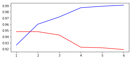
결과를 보니검증 성능이 epoch이 증가할 수록 떨어지는 것으로 보아 모델이 과대적합 된 듯 함. dropout 비율을 더 높이거나, 레이어 수를 줄여야 할 것 같음.
Predict test set
## predict test_set
test_pred = model.predict(pad_test)
7. submit submission.csv
sample_result = pd.DataFrame()
sample_result['id'] = test_df.index
sample_result['prediction'] = test_pred

## submit sample_submission.csv
sample_result.to_csv('submission.csv', index=False)
Outro
최종 제출 결과 91.1% 라는 검증 결과가 나와 상위 84%.... 문제를 제대로 이해를 안하고 시작해서 그런지 모델 수정으로는 이 이상 성능 향상이 되지 않았다. 다른 상위 커널을 살펴보니 대부분 feature engineering부분에서 텍스트 처리에 많은 노력을 기울인 것 같다.
더 수정해서 해보려고 했는데, 제출 기간이 아쉽게 종료가 되어 더 진행해보지는 않았다.
최근 정권우님이 쓰신 '머신러닝 탐구생활'이라는 책을 구매하였는데, 다양한 kaggle문제를 어떻게 접근해야 하는지, 또 최근 kaggle내에서 어떤 모델이 주로 사용되는지 트렌드를 살펴볼 수 있을 것 같아 열심히 읽어보는 중이다. 완독 후 다시 다른 캐글 문제에 도전해봐야겠다!
.jpeg)