Classification in Machine Learning - Decision Tree

Brief Summay
A supervised learning is a machine learning task of learning a function that maps an input to an output based on example input-output pairs. Classification, one of the most famous supervised learning classification techniques, trains its machine learning algorithm based on the given feature and label datasets and predicts the unknown lablel data in the test set.

Types of Machine Learning Classification Algorithm

• Naive Bayes Classifier
• Logistic Regression
• Decision Tree Classifier
• Support Vector Machine
• Nearest Neighbor Algorithm
• Neural Network
• Ensemble Method Combining Same or Different Algorithms

On this post, we will be studying about Ensemble Method. However, before doing so we will first delve into Decision Tree, which is often used as a weak-learner for Ensemble method.

Decision Tree

Decision Tree is one of the most intuitive ML-algorithm. The model automatically finds the pattern within the data and establishes a classification principle based on a tree-structure. It is a recursive implementations of if - else condition until the model satisfies the constraints.

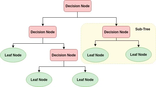
Diagram above shows the basic structure of the Deision Tree. Decision Tree starts from the Root Node, the very fist node of the tree. The nodes derived from the root node becomes Sub Tree which is composed of Decision Node and Leaf Node. Decision Node becomes the condition of decision and the Leaf Node is the classified result of the decision.

In order to classify data with least amount of decision node, it is important to create a condition to contain as much as data as possible. In other words, it is significant to split tree with high data uniformity.

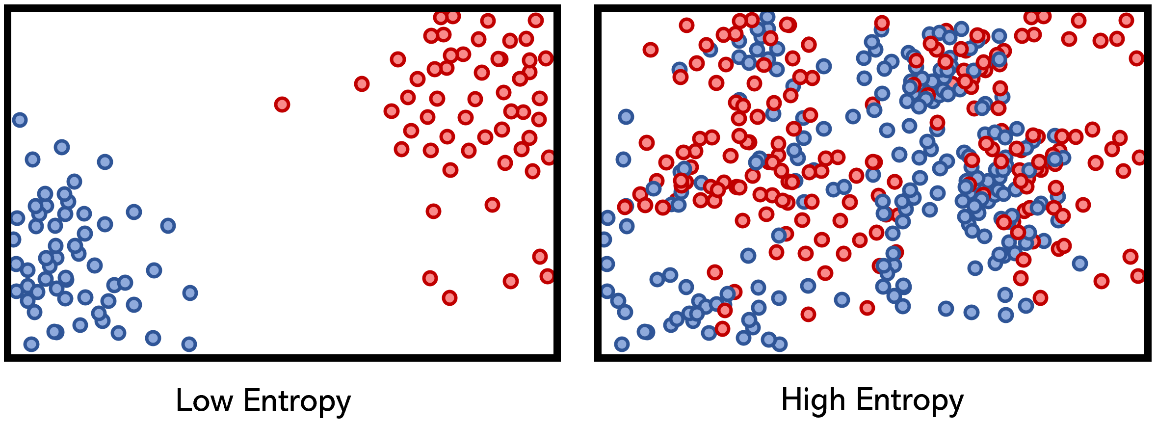
Information Gain based on entropy and Gini Coefficient are often used in measuring the uniformity of the dataset.

• Entropy is the measure of the disorder or uncertainty of the data. Higher the disorder, higher the entropy, and lower the disorder, lower the entropy value. Information Gain equals 1 - entropy. Decision Tree classifies data based on higher Information Gain score.

• Gini Coefficient also measures the disorder or uncertainty of the data. Higher the coefficient, higher the unorder is. Hence, the Decision Tree Classifier classifies dataset based on low Gini Coefficient.

Characteristics of Decision Tree

Advantage of Decision Tree comes from its intuitiveness. Since the Decision Tree soley cares about uniformity, there is no need for feature-scaling or data-preprocessings (ex- standardization, normalization).

However, weakness of Decision Tree is that there is a high chance of undermining accuracy due to overfitting. Since the tree recursively creates different sub-trees to satisfy the condtion, the tree become inevitably deep and complex. Therefore, it is sometimes better to set a constraint to the tree model to enhance the performance.

Visualization of Tree Model

Using Graphviz package, we will be visualizing the tree model.

Install Graphviz

Input

from sklearn.tree import DecisionTreeClassifier
from sklearn.datasets import load_iris
from sklearn.model_selection import train_test_split
import warnings
warnings.filterwarnings('ignore')

dt_clf = DecisionTreeClassifier(random_state=156)
t
iris_data = load_iris()
X_train , X_test , y_train , y_test = train_test_split(iris_data.data, iris_data.target,
                                                       test_size=0.2,  random_state=11)

dt_clf.fit(X_train , y_train)

Input

from sklearn.tree import export_graphviz

export_graphviz(dt_clf, out_file="tree.dot", class_names=iris_data.target_names , \
feature_names = iris_data.feature_names, impurity=True, filled=True)

import graphviz

with open("tree.dot") as f:
    dot_graph = f.read()
graphviz.Source(dot_graph)

Output

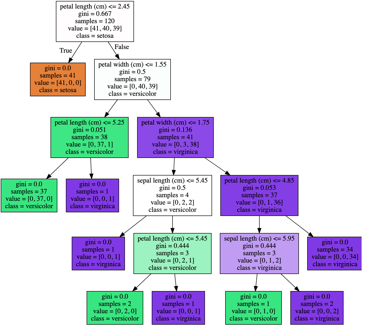
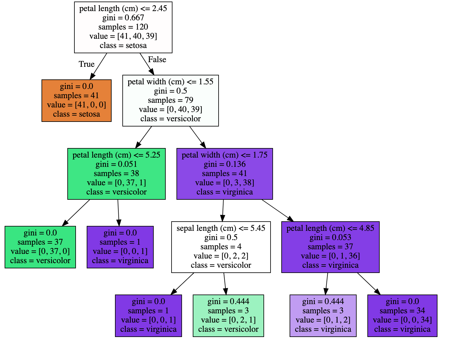
We can see that the Decision Tree has extended itself until it satifies every label data. Such complexity might show high accuracy for train data-set. However, it has an high chance of falsely predicting to test data-set. Now, let us limit the maximum depth of Decision Tree to 3.

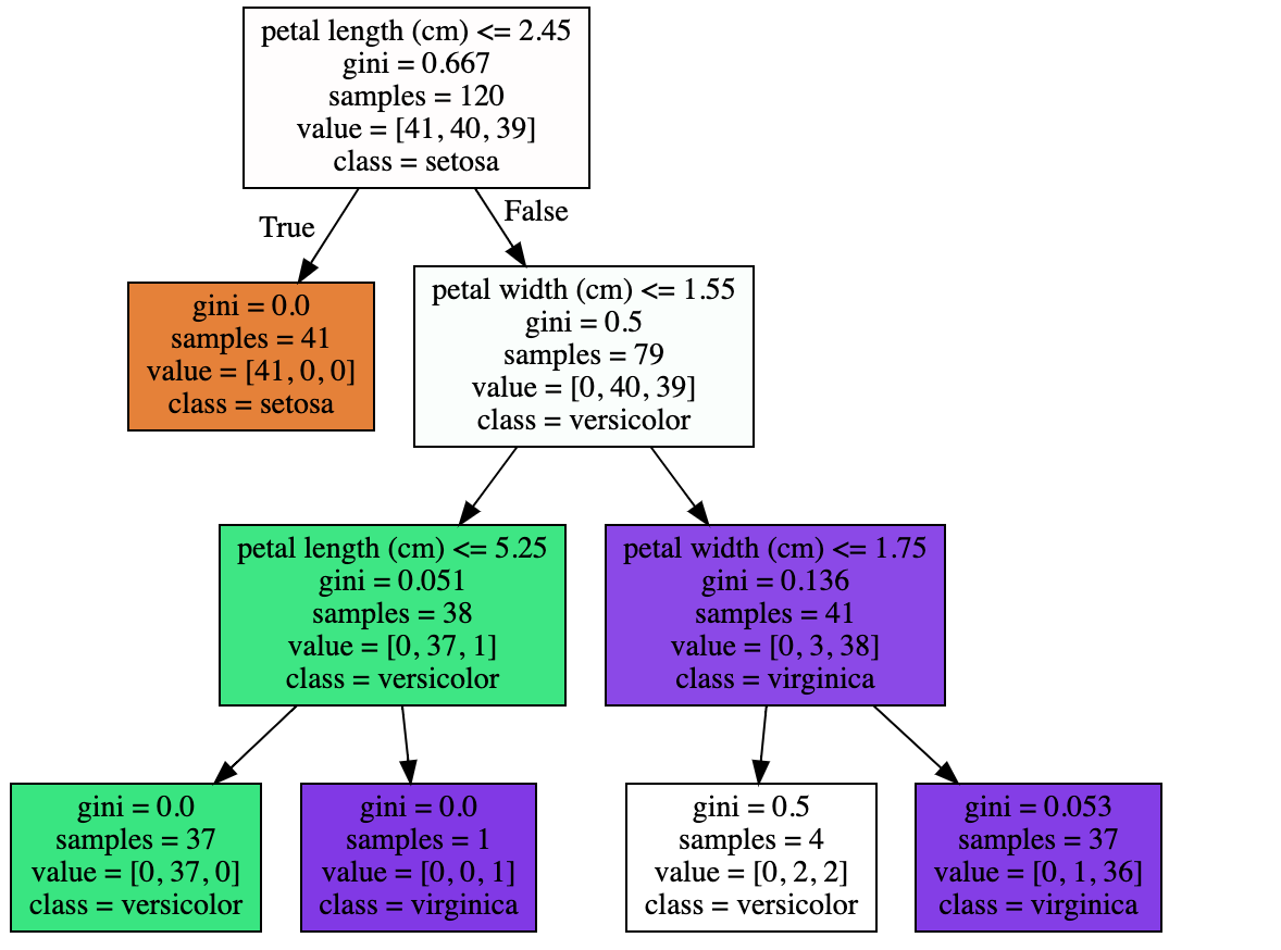
Input (max_depth)

from sklearn.tree import export_graphviz
import graphviz

dt_clf = DecisionTreeClassifier(random_state=156, max_depth=3)

iris_data = load_iris()
X_train , X_test , y_train , y_test = train_test_split(iris_data.data, iris_data.target,
                                                       test_size=0.2,  random_state=11)

dt_clf.fit(X_train , y_train)


export_graphviz(dt_clf, out_file="tree.dot", class_names=iris_data.target_names , \
feature_names = iris_data.feature_names, impurity=True, filled=True)

with open("tree.dot") as f:
    dot_graph = f.read()
graphviz.Source(dot_graph)

Output

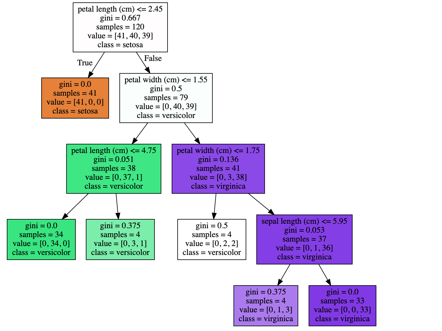
Input (min_sampples_split)

from sklearn.tree import export_graphviz
import graphviz

dt_clf = DecisionTreeClassifier(random_state=156, min_samples_split=4)

iris_data = load_iris()
X_train , X_test , y_train , y_test = train_test_split(iris_data.data, iris_data.target,
                                                       test_size=0.2,  random_state=11)

dt_clf.fit(X_train , y_train)


export_graphviz(dt_clf, out_file="tree.dot", class_names=iris_data.target_names , \
feature_names = iris_data.feature_names, impurity=True, filled=True)

with open("tree.dot") as f:
    dot_graph = f.read()
graphviz.Source(dot_graph)

Output

Input (min_samples_leaf)

from sklearn.tree import export_graphviz
import graphviz

dt_clf = DecisionTreeClassifier(random_state=156, min_samples_leaf=4)

iris_data = load_iris()
X_train , X_test , y_train , y_test = train_test_split(iris_data.data, iris_data.target,
                                                       test_size=0.2,  random_state=11)

dt_clf.fit(X_train , y_train)


export_graphviz(dt_clf, out_file="tree.dot", class_names=iris_data.target_names , \
feature_names = iris_data.feature_names, impurity=True, filled=True)

with open("tree.dot") as f:
    dot_graph = f.read()
graphviz.Source(dot_graph)

Output

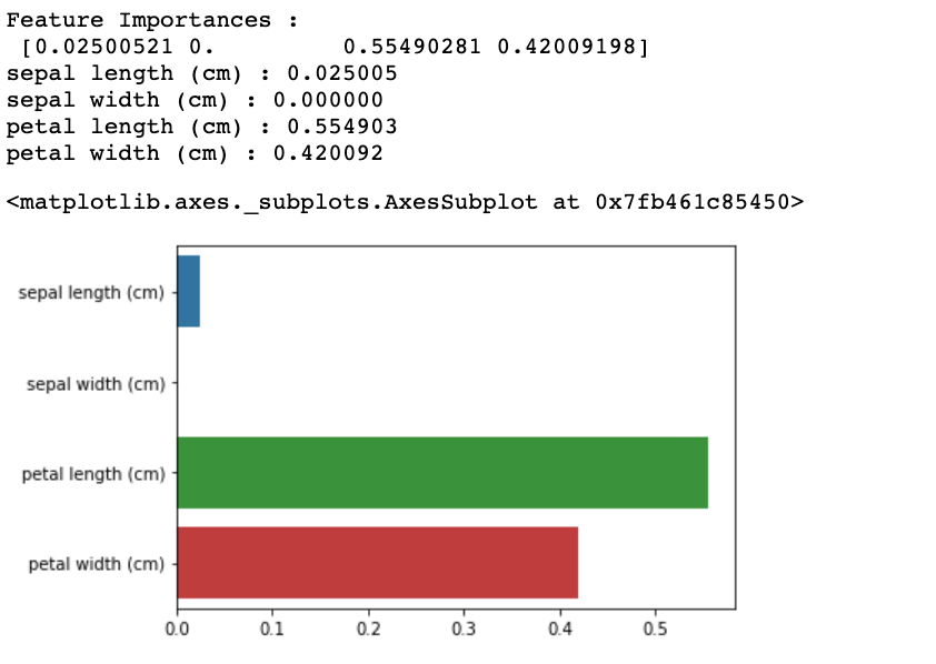
Now, we will use feature_importances to see which features had the most impact on classification.

Input

dt_clf = DecisionTreeClassifier(random_state=156)

iris_data = load_iris()
X_train , X_test , y_train , y_test = train_test_split(iris_data.data, iris_data.target,
                                                       test_size=0.2,  random_state=11)

dt_clf.fit(X_train , y_train)

Input

import seaborn as sns
import numpy as np
%matplotlib inline

print('Feature Importances : \n', dt_clf.feature_importances_)

for name, value in zip(iris_data.feature_names, dt_clf.feature_importances_):
    print('{0} : {1:3f}'.format(name, value))
    
sns.barplot(x=dt_clf.feature_importances_, y=iris_data.feature_names)

Output