Today, we will be using decision tree to perform classification prediction on UCI Machine Learning Repository's Human Activity Recognition dataset. The dataset is a compilation of various feature data collected after installing smartphone sensor to 30-participants. Based on the collected feature-set we will classify the type of action by each participant.
After clicking Data Folder download UCI HAR Dataset.zip and change its name to human_activity.
Now that we have downloaded the dataset, we will begin the preprocessing of the data.
Input
# UCI Human Activity Recognition Using Smartphones
import pandas as pd
import matplotlib.pyplot as plt
%matplotlib inline

features_name_df = pd.read_csv('./human_activity/features.txt', sep='\s+',
                               header=None, names=['column_index', 'column_name'])

feature_name = feature_name_df.iloc[:, 1].values.tolist()

print('Extract 10 Feature Names : \n', feature_name[:10])
Output
Extract 10 Feature Names :
 ['tBodyAcc-mean()-X', 'tBodyAcc-mean()-Y', 'tBodyAcc-mean()-Z', 'tBodyAcc-std()-X', 'tBodyAcc-std()-Y', 'tBodyAcc-std()-Z', 'tBodyAcc-mad()-X', 'tBodyAcc-mad()-Y', 'tBodyAcc-mad()-Z', 'tBodyAcc-max()-X']
Now let us check whether or not there are duplicate column names.
Input
feature_dup_df = feature_name_df.groupby('column_name').count()

print(feature_dup_df[feature_dup_df['column_index'] > 1].count())
feature_dup_df[feature_dup_df['column_index'] > 1].head()
Output
column_index    42
dtype: int64

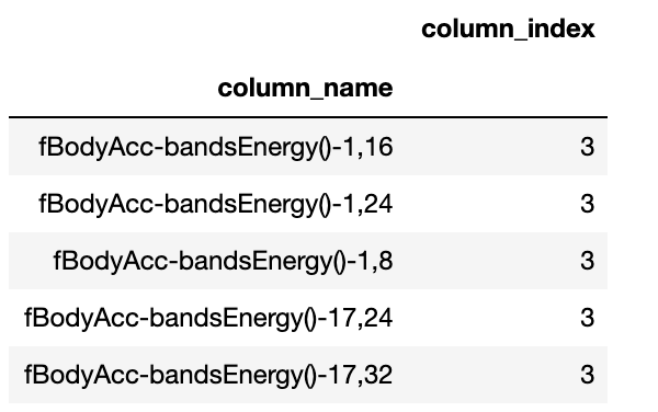
There are total 42 duplicate feature-names, we will simply add _1 or _2 to initial feature names to create distinctive values.
Input
def get_new_feature_name_df(old_feature_name_df):
    feature_dup_df = pd.DataFrame(data=old_feature_name_df.groupby('column_name').cumcount(),
                                     columns=['dup_cnt'])

    feature_dup_df = feature_dup_df.reset_index()

    new_feature_name_df = pd.merge(old_feature_name_df.reset_index(), feature_dup_df, how='outer')
    new_feature_name_df['column_name'] = new_feature_name_df[['column_name', 'dup_cnt']].apply(lambda x: x[0]+'_'+str(x[1])
                                                                                                  if x[1] > 0 else x[0], axis=1)

    new_feature_name_df = new_feature_name_df.drop(['index'], axis=1)

    return new_feature_name_df
Now, we will create a function to manage dataset.
Input
import pandas as pd

def get_human_dataset( ):

    feature_name_df = pd.read_csv('./human_activity/features.txt',sep='\s+',
                        header=None,names=['column_index','column_name'])

    new_feature_name_df = get_new_feature_name_df(feature_name_df)

    feature_name = new_feature_name_df.iloc[:, 1].values.tolist()

    X_train = pd.read_csv('./human_activity/train/X_train.txt',sep='\s+', names=feature_name )
    X_test = pd.read_csv('./human_activity/test/X_test.txt',sep='\s+', names=feature_name)

    y_train = pd.read_csv('./human_activity/train/y_train.txt',sep='\s+',header=None,names=['action'])
    y_test = pd.read_csv('./human_activity/test/y_test.txt',sep='\s+',header=None,names=['action'])

    return X_train, X_test, y_train, y_test


X_train, X_test, y_train, y_test = get_human_dataset()
Input
print('### Train Dataset Info \n')
print(X_train.info())
Output
### Train Dataset Info

<class 'pandas.core.frame.DataFrame'>
RangeIndex: 7352 entries, 0 to 7351
Columns: 561 entries, tBodyAcc-mean()-X to angle(Z,gravityMean)
dtypes: float64(561)
memory usage: 31.5 MB
None
There are total 561 float-type feature data which do not need any categorical encoding.
Input
print(y_train['action'].value_counts())Output
6    1407
5    1374
4    1286
1    1226
2    1073
3     986
Name: action, dtype: int64
Label data are fairly distributed without any bias.
Now, we will use DecisionTreeClassifier to classify the activity. We will set the hyper-parameters to default value and extract those afterwards.
Input
from sklearn.tree import DecisionTreeClassifier
from sklearn.metrics import accuracy_score

dt_clf = DecisionTreeClassifier(random_state=156)
dt_clf.fit(X_train, y_train)

pred = dt_clf.predict(X_test)
accuracy = accuracy_score(y_test, pred)
print('Accuracy of DecisionTreeClassifier : {0:4f} \n'.format(accuracy))

# extract hyper parameter of DecisionTreeClassifier
print('DecisionTreeClassifier Hyper Parameter : \n', dt_clf.get_params())
Output
Accuracy of DecisionTreeClassifier : 0.854768

DecisionTreeClassifier Hyper Parameter :
 {'class_weight': None, 'criterion': 'gini', 'max_depth': None, 'max_features': None, 'max_leaf_nodes': None, 'min_impurity_decrease': 0.0, 'min_impurity_split': None, 'min_samples_leaf': 1, 'min_samples_split': 2, 'min_weight_fraction_leaf': 0.0, 'presort': False, 'random_state': 156, 'splitter': 'best'}
The result has 85.48% of accuracy. Now we will see how the tree-depth of Decision Tree influences the accuracy of the model. We studied previously that the tree extends its depth until the tree satisfies the condition. Hence, we will gradually change the maximum depth of the tree to and observe the shift in accuracy.
Input
from sklearn.model_selection import GridSearchCV

params = {
    'max_depth' : [6,8,10,12,16,20,24]
}

grid_cv = GridSearchCV(dt_clf, param_grid=params, scoring='accuracy', cv=5, verbose=1)
grid_cv.fit(X_train, y_train)

print('GridSearchCV Best Accuracy Score : {0:4f}'.format(grid_cv.best_score_))
print('GridSearchCV Best Hyperparamter : ', grid_cv.best_params_)
Output
GridSearchCV Best Accuracy Score : 0.852557
GridSearchCV Best Hyperparamter :  {'max_depth': 8}
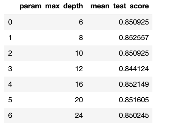
GridSearchCV returns that the best hyper parameter is at maximum depth of 8 with accuracy of 85.26%. We will see how the accuracy changed based on the change in CV set.
Using GridSearchCV's cvresults, we will extract the mean test score of each steps.
Input
cv_results_df = pd.DataFrame(grid_cv.cv_results_)

cv_results_df[['param_max_depth', 'mean_test_score']]

Using the result from GridSearchCV, we will estimate the accuracy of the Decision Tree in separate train-set.
Input
max_depths = [6,8,10,12,16,20,24]

for depth in max_depths:
    dt_clf = DecisionTreeClassifier(max_depth=depth, random_state=156)
    dt_clf.fit(X_train, y_train)

    pred = dt_clf.predict(X_test)
    accuracy = accuracy_score(y_test, pred)

    print('{0} Max Depth Accuracy {1:4f}'.format(depth, accuracy))
Output
6 Max Depth Accuracy 0.855786
8 Max Depth Accuracy 0.870716
10 Max Depth Accuracy 0.867323
12 Max Depth Accuracy 0.864608
16 Max Depth Accuracy 0.857482
20 Max Depth Accuracy 0.854768
24 Max Depth Accuracy 0.854768
As we have expected, maximum depth at 8 returns the highest accuracy score of 87.07%.
Now, let us also try tuning the accuracy by changing minimum amount of samples to split the leaf-node.
Input
params = {
    'max_depth' : [8,12,16,20],
    'min_samples_split' : [16,24],
}

grid_cv = GridSearchCV(dt_clf, param_grid=params, scoring='accuracy', cv=5, verbose=1)
grid_cv.fit(X_train, y_train)

print('Grid Search CV Best Accuracy : {0:4f}'.format(grid_cv.best_score_))
print('Grid Search Best Hyper Parameter : ', grid_cv.best_params_)
Output
Grid Search CV Best Accuracy : 0.855005
Grid Search Best Hyper Parameter :  {'max_depth': 8, 'min_samples_split': 16}
Now, we will use identical trained estimator to perform classification in separate test-set.
Input
best_dt_clf = grid_cv.best_estimator_
pred1 = best_dt_clf.predict(X_test)
accuracy = accuracy_score(y_test, pred1)

print('Decision Tree Classifier Accuracy {0:4f}'.format(accuracy))
Output
Decision Tree Classifier Accuracy 0.871734
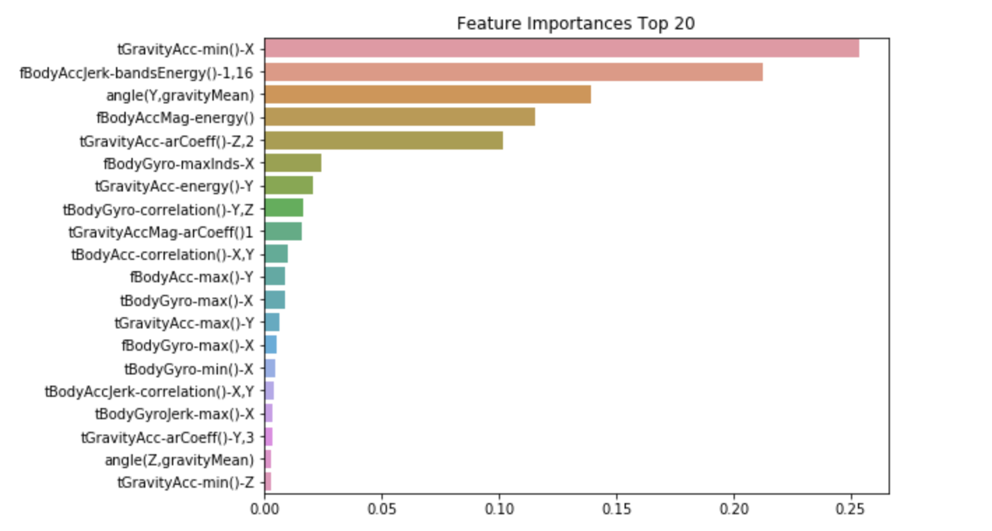
Now using barplot, we will visualize the importances of feature in the model.
Input
import seaborn as sns

ftr_importances_values = best_df_clf.feature_importances_

ftr_importances = pd.Series(ftr_importances_values, index=X_train.columns)
ftr_top20 = ftr_importances.sort_values(ascending=False)[:20]

plt.figure(figsize=(8,6))
plt.title('Feature Importances Top 20')

sns.barplot(x=ftr_top20, y=ftr_top20.index)
plt.show()
Output

