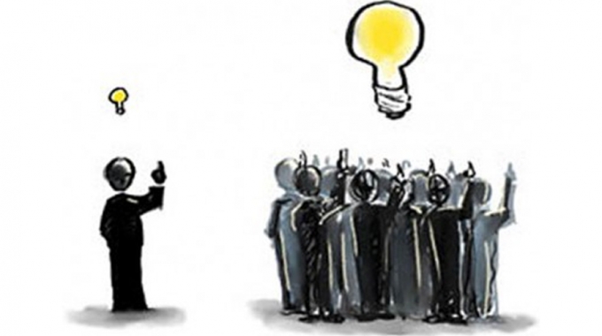
Ensemble Learning : Voting and Bagging

Ensemble Learning : process by which multiple models, such as classifiers or experts, are strategically generated and combined to solve a particular computational intelligence problem.

Although, deep learning is prominently favored by data-scientists in classfication of unstructured-data (i.e. - image, video, voice), ensemble learning shows outstanding performance in classification of structured-data.

Algorithms such as Random Forest and Gradient Boosting have been widely used by data-scientists. And now, new algorithms such as XGBoost, LightGBM and Stacking are gaining popularity due to their classification performances.

Ensemble Learning is mainly divided into three ways - Voting, Bagging, and Boosting. Voting and Bagging are deciding the final result by combining multiple classifiers.

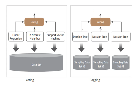
Voting

• Generally combine different classifiers
• Classifiers use identical dataset

Bagging

• Generally use identical classifiers
• Classifiers use different datasets

Diagram on the left is Voting Algorithm. Three different classifiers (Linear Regression, K-Nearest Neighbor & Support Vector Machine) performs training on identical data-set and decide on final result through voting.

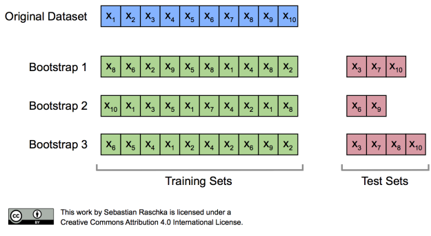
Bagging Algorithm on the right combines identical ML-algorithm Decision Tree on each classifier. Afterwards, each classifier use different extracted dataset from the original set - also known as the bootstrapping method. Different to cross-validation which does not allow use of duplicate sample data, bootstrapping allows nesting on use of data.

Hard Voting vs. Soft Voting

There are two ways in voting procedure. Classification by hard-voting is like Winner Take All system. Out of multiple outputs produced by the classifiers, the majority output is chosen to be the final result of the model.

In contrast, soft-voting is a voting process which every classifiers' outputs are taken into account. Soft-voting sums the predicted probabilities for class lables and returns the final classification with the largest sum probability.

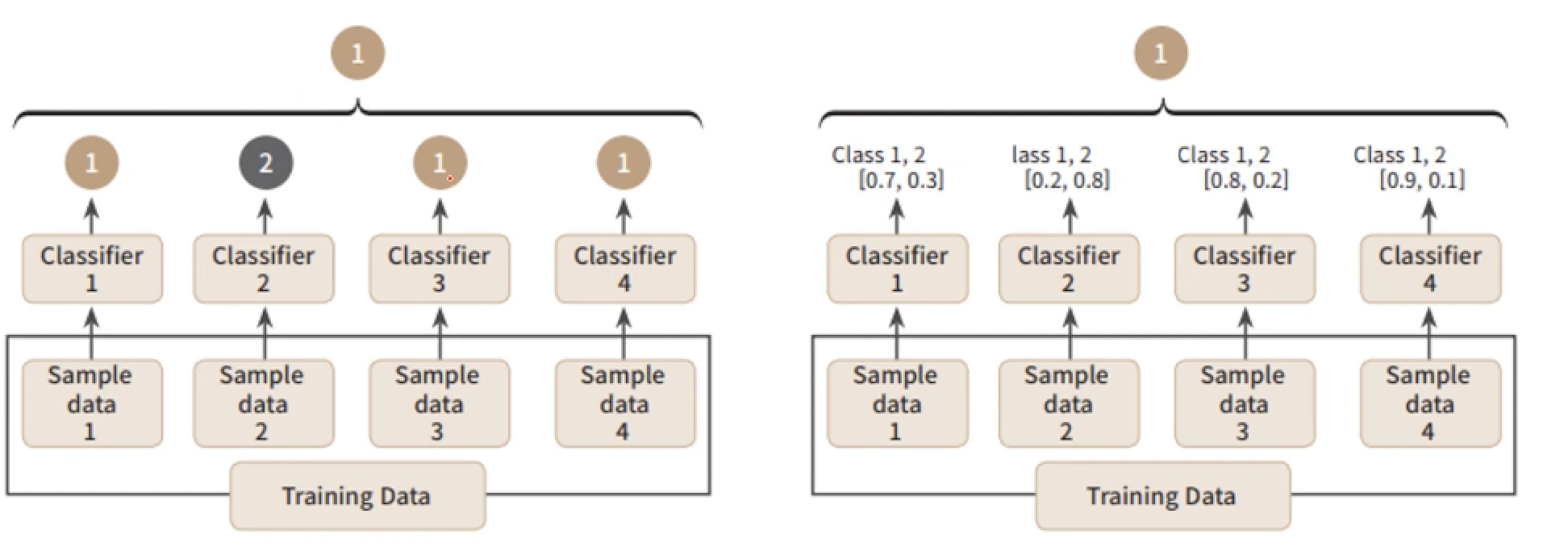
                		< Hard Voting vs. Soft Voting>

Voting Classifier

We will be using Wisconsin Breast Cancer dataset to try out Voting Classifier. We will be making the classifier based off of Logistci Regresseion and KNN models.

Input

import pandas as pd 

from sklearn.ensemble import VotingClassifier
from sklearn.linear_model import LogisticRegression
from sklearn.neighbors import KNeighborsClassifier
from sklearn.datasets import load_breast_cancer
from sklearn.model_selection import train_test_split
from sklearn.metrics import accuracy_score

cancer = load_breast_cancer()

data_df = pd.DataFrame(cancer.data, columns=cancer.feature_names)

data_df.head(3)

Output

Now, we will create Logistic and KNN soft-voting classifiers. Voting Classifier receives estimator and voting-value as parameters.

• Estimator : multiple classifiers which will be used for voting in tuple-list type
• Voting : type of voting (i.e. - hard voting, soft voting)

Input

lr_clf = LogisticRegression()
knn_clf = KNeighborsClassifier(n_neighbors=8)

vo_clf = VotingClassifier(estimators=[('LR', lr_clf), ('KNN', knn_clf)], voting='soft')

X_train, X_test, y_train, y_test = train_test_split(cancer.data, cancer.target, test_size=0.2, random_state=156)

vo_clf.fit(X_train, y_train)
pred = vo_clf.predict(X_test)
print('Voting Classifier Accuracy : {0:4f} \n'.format(accuracy_score(y_test, pred)))

classifiers = [lr_clf, knn_clf]

for classifier in classifiers: 
    classifier.fit(X_train, y_train)
    pred = classifier.predict(X_test)
    class_name = classifier.__class__.__name__

    print('{0} Classifier Accuracy {1} \n'.format(class_name, accuracy_score(y_test, pred)))
    

Output

Voting Classifier Accuracy : 0.956140 

LogisticRegression Classifier Accuracy 0.9473684210526315 

KNeighborsClassifier Classifier Accuracy 0.9385964912280702 

Bagging (Random Forest)

Bagging is creating multiple classifiers with identical algorithm to decide final class value. Random Forest is one of the most famous model which uses bagging algorithm. It relatively has a fast execution speed and returns outstanding performance in various fields.

In Random Forest, multiple Decision Trees extract individual samples from the entire data-set and execute training. Each sample which the classifiers train is nested-samples which in other words mean the data are not exclusive. Such method is better known as bootstrapping (Term Bagging is derived from boostrap aggregating).

Input

import pandas as pd
import warnings 
warnings.filterwarnings('ignore')

def get_new_feature_name_df(old_feature_name_df):
    feature_dup_df = pd.DataFrame(data=old_feature_name_df.groupby('column_name').cumcount(),
                                     columns=['dup_cnt'])

    feature_dup_df = feature_dup_df.reset_index()

    new_feature_name_df = pd.merge(old_feature_name_df.reset_index(), feature_dup_df, how='outer')
    new_feature_name_df['column_name'] = new_feature_name_df[['column_name', 'dup_cnt']].apply(lambda x: x[0]+'_'+str(x[1])
                                                                                                  if x[1] > 0 else x[0], axis=1)

    new_feature_name_df = new_feature_name_df.drop(['index'], axis=1)
    
    return new_feature_name_df

def get_human_dataset( ):
    
    feature_name_df = pd.read_csv('./human_activity/features.txt',sep='\s+',
                        header=None,names=['column_index','column_name'])
    
    new_feature_name_df = get_new_feature_name_df(feature_name_df)
    
    feature_name = new_feature_name_df.iloc[:, 1].values.tolist()
    
    X_train = pd.read_csv('./human_activity/train/X_train.txt',sep='\s+', names=feature_name )
    X_test = pd.read_csv('./human_activity/test/X_test.txt',sep='\s+', names=feature_name)
    
    y_train = pd.read_csv('./human_activity/train/y_train.txt',sep='\s+',header=None,names=['action'])
    y_test = pd.read_csv('./human_activity/test/y_test.txt',sep='\s+',header=None,names=['action'])
    
    return X_train, X_test, y_train, y_test


X_train, X_test, y_train, y_test = get_human_dataset()

Now that we have finished data-preprocessing of human-activity data, we will create Random Forest Classifier.

Input

from sklearn.ensemble import RandomForestClassifier
from sklearn.metrics import accuracy_score

X_train, X_test, y_train, y_test = get_human_dataset()

rf_clf = RandomForestClassifier(random_state=0)
rf_clf.fit(X_train, y_train)

pred = rf_clf.predict(X_test)
accuracy = accuracy_score(y_test, pred)
print('Accuracy of Random Forest : {0:4f}'.format(accuracy))

Output

Accuracy of Random Forest : 0.910757

Tree model Ensemble Learning's weakness comes from the fact that there are too much hyper-parameters to adjust and that the model is time consuming.

We will use GridSearchCV to adjust the hyper parameter. We will be setting n_estimators equal to 100 and CV to 2.

Input

from sklearn.model_selection import GridSearchCV 

params = {
    'n_estimators' : [100],
    'max_depth' : [6, 8, 10, 12],
    'min_samples_leaf' : [8, 12, 18],
    'min_samples_split' : [8, 16, 20]
}

rf_clf = RandomForestClassifier(random_state=0, n_jobs=1)
grid_cv = GridSearchCV(rf_clf, param_grid=params, cv=2, n_jobs=1)
grid_cv.fit(X_train, y_train)

print('Best Hyper Parameter : ', grid_cv.best_params_)
print('Best Accuracy : {0:4f}'.format(grid_cv.best_score_))

Output

Best Hyper Parameter :  {'max_depth': 10, 'min_samples_leaf': 8, 'min_samples_split': 8, 'n_estimators': 100}
Best Accuracy : 0.916621

Input

rf_clf1 = RandomForestClassifier(n_estimators=300, max_depth=10, min_samples_leaf=8, \
                                 min_samples_split=8, random_state=0)
rf_clf1.fit(X_train , y_train)
pred = rf_clf1.predict(X_test)
print('Accuracy : {0:.4f}'.format(accuracy_score(y_test , pred)))

Output

Accuracy : 0.9165

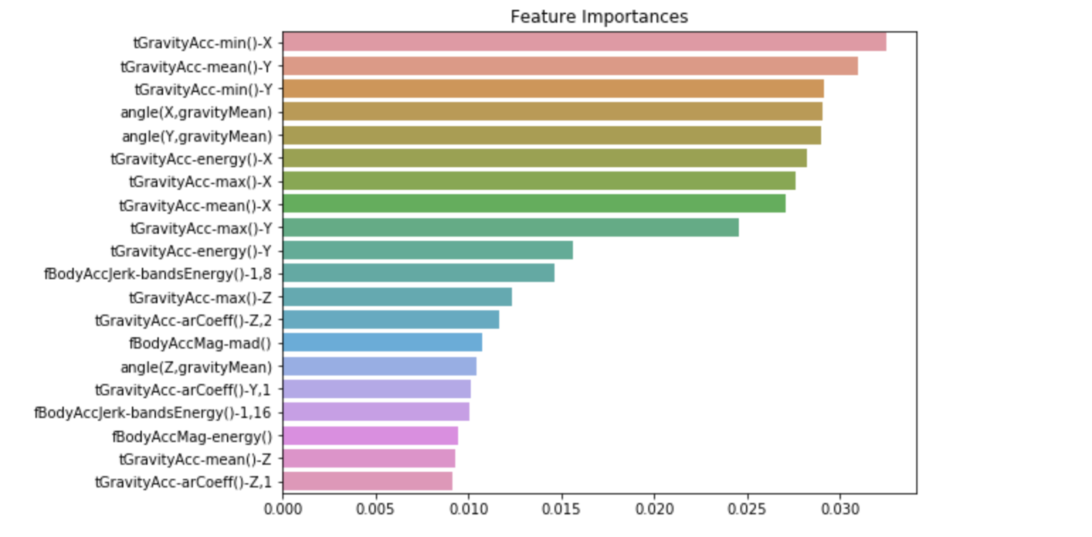
Now, we will visualize the importances of feature-data within the model.

Input

import matplotlib.pyplot as plt
import seaborn as sns 
%matplotlib inline 

ftr_importances_values = rf_clf1.feature_importances_
ftr_importances = pd.Series(ftr_importances_values, index=X_train.columns)
ftr_top20 = ftr_importances.sort_values(ascending=False)[:20]

plt.figure(figsize=(8, 6))
plt.title('Feature Importances')
sns.barplot(x=ftr_top20, y=ftr_top20.index)

plt.show()

Output