Bayesian Estimation을 설명하기 위한 몇가지 이론들을 먼저 보자.
Hidden Markov Model (HMM)
Measurement Model
Example. Door open?
문이 하나 존재하고, 문의 상태를 X, 센서의 관측을 Z라 하면
X={open , closed}Z={sensor_open , sensor_closed}
다음처럼 나타낼 수 있다.
문은 외력이 작용하지 않는다고 하고, 센서의 성능은 다음과 같다고 하자.
p(sensor_open∣open)=0.7,p(sensor_open∣closed)=0.2p(sensor_closed∣open)=0.3 p(sensor_closed∣closed)=0.8
이제 처음에 문의 상태를 모르므로 uniform하게 확률을 설정하고, 우리가 구해야 하는 것은 센서가 열렸다는 관측이 주어졌을때, 실제로 문이 열렸는지를 알고 싶은것이다.
그렇다면 베이즈 룰에 의해 다음과 같은 식을 얻을 수 있다.
p(xj∣z)=∑i=1np(z∣xi)p(xi)p(z∣xi)p(xj)=η ⋅p(z∣xj)p(xj)
위의 식에 아까의 확률을 곱하여 계산해보면 센서 관측이 열렸다고 주어졌을때, 실제로 문이 열렸을 확률 p(open∣sensor_open)=97 임을 알 수 있다.
이를 간단하게 행렬 계산으로도 나타낼 수 있다
[0.7×0.50.2×0.50.3×0.50.8×0.5]=([0.70.30.20.8]T)⊙[0.50.5]
그리고 1열의 결과를 normalize하면 된다.
여기서, 센서의 성능에 따라 결정되는 행렬을 Measurement Model 이라고 한다.
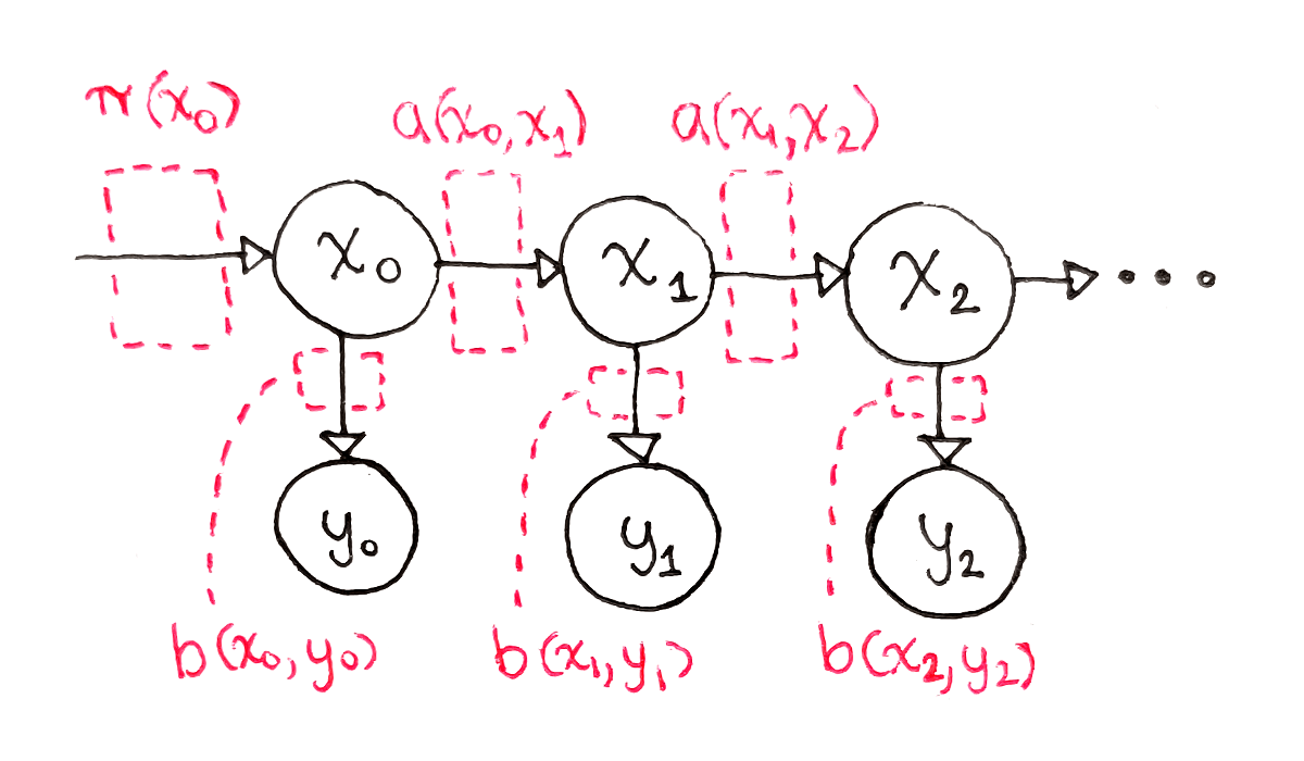
아마 이 그림이 HMM을 가장 잘 표현하는 그림일 것이다.
여기서는 중요한 2가지 가정이 존재한다.
- 현재 상태 xt는 이전상태 xt−1과 현재 control ut 에 stochastically dependent 하다.
- 현재 관측 zt는 현재 상태 xt에만 stochastically dependent 하다.
HMM에는 여러가지 경우가 있는데, 먼저 위에서 예제로 보았던 Measurement model만 있는 경우를 먼저 보겠다.
HMM : only measurement model
아까의 예시에서 좀더 나아가, 이번엔 센서의 관측이 2번 들어온다고 해보자
p(open∣sensor_open , sensor_open)
예를 들자면 이러한 경우이다.
여기서 HMM의 강력한 점이 등장하는데, 오직 현재 상태는 이전 상태에만 dependent하기 때문에,
p(open∣sensor_open , sensor_open)=p(open∣sensor_open)
이렇게 된다는 것이다.
HMM : Measurement Model + State Transition without Contorl
HMM에 시간에 따른 State Transition (xt)과 Measurement (zt) 가 있는 경우이다.
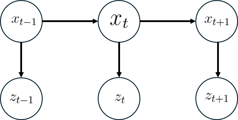
- x1에서 x2로 state transition이 일어났고, 그때의 관측을 z2,z1 이라 하면,
p(x2∣z2,z1)==η2 p(z2∣x2,z1)p(x2∣z1)η2 1p(z2∣x2)2p(x2∣z1)
이다. 여기서 1번식은 measurement model로 아는 값이고, 2번식은 다음처럼 구할 수 있다.
p(x2∣z1)==x1∑p(x2∣x1,z1)p(x1∣z1)x1∑p(x2∣x1)p(x1∣z1)
Bayesian Estimation
- 시간 t에 대해, state trensition과 Measurement가 모두 존재할때, 다음처럼 recursive한 관계가 성립한다.
p(x0)=p(x1∣z1)=p(x2∣,z2,z1)=⋮=p(xt∣,zt,zt−1,⋯,z1)=Typically assumped uniform distributionη1 ⋅p(z1∣x1)x0∑p(x1∣x0)p(x0)η2 ⋅p(z2∣x2)x1∑p(x2∣x1)p(x1∣z1)⋮ηt ⋅p(zt∣xt)xt−1∑p(xt∣xt−1)p(xt−1∣zt−1,zt−2,⋯,z1)
HMM : Transition model + State Transition model with Control
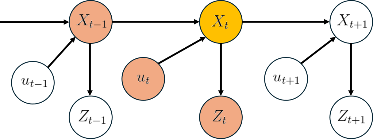
위의 recursive한 식에, u를 conditioning random variable로 포함시키면 아래와 같은 식을 얻을 수 있다.
p(xt∣zt,⋯,z1,ut,⋯,u1)=ηt⋅p(zt∣xt,ut)xt−1∑p(xt∣xt−1,ut)p(xt−1∣zt−1,⋯,z1,ut−1,⋯,u1)=ηt⋅p(zt∣xt)xt−1∑p(xt∣xt−1,ut)p(xt−1∣zt−1,⋯,z1,ut−1,⋯,u1)
위의 식을 bel(xt)를 써서 정리하게 된다면, 다음과 같다.
bel(xt)=p(xt∣z1,⋯,zt,u1,⋯,ut)=ηt⋅p(zt∣xt)⋅bel(xt)
where
bel(xt)=xt−1∑p(xt∣xt−1,ut)p(xt−1∣z1,⋯,zt−1,u1,⋯,ut−1)=xt−1∑p(xt∣xt−1,ut)bel(xt−1)
두 식을 하나로 합치면 아래와 같이 recursive한 형태로 표현된다.
bel(xt)=ηt⋅p(zt∣xt)⋅xt−1∑p(xt∣xt−1,ut)bel(xt−1) 