Approximation-generalization tradeoff
우리의 목적은 out of sample error, 즉 Eout이 낮은 learner을 얻고자 하는 것이다.
이 learner을 얻기 위해서는 우리가 2가지 방법을 생각할 수 있다.
과연 우리가 모델을 더 복잡하게 만들것이냐, 아니면 hypothesis를 좀더 일반화할것이냐에 따라 달렸다.
그렇다면 우리가 만들어야 하는 f는 얼마나 hypothesis를 잘 예측하는지와, 주변을 얼마나 잘 cover하는지를 따져야 한다.
out of sample error부터 시작해보자.
아래의 수식에서 D는 data set이고, g는 candidate of best hypothesis이다.
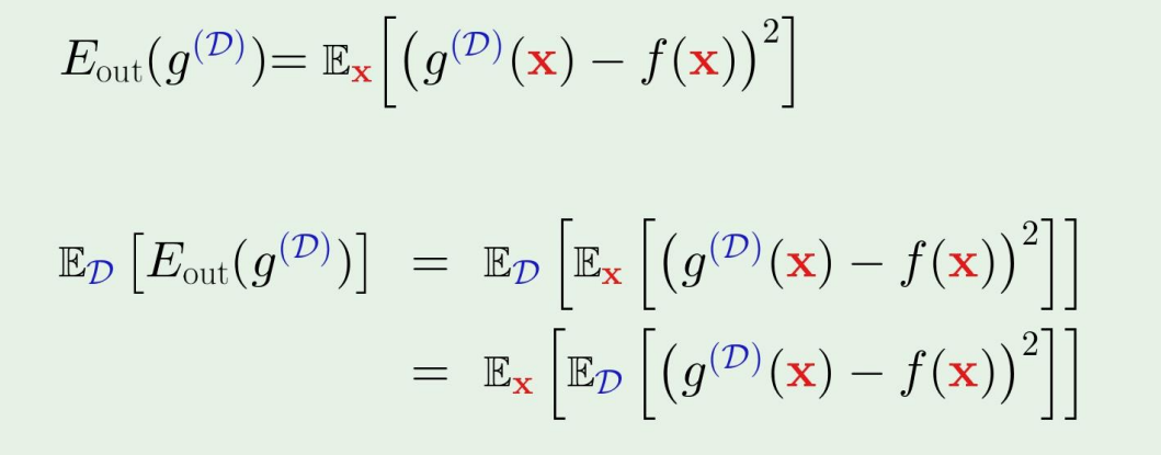
Eout는 내 data set에 dependent 하므로 위의 수식에서 아래처럼 쓸수있고, 맨 마지막줄의 ED[g(D)(x)−f(x)2]는 data set에 대한 out of sample error의 expectation이다.
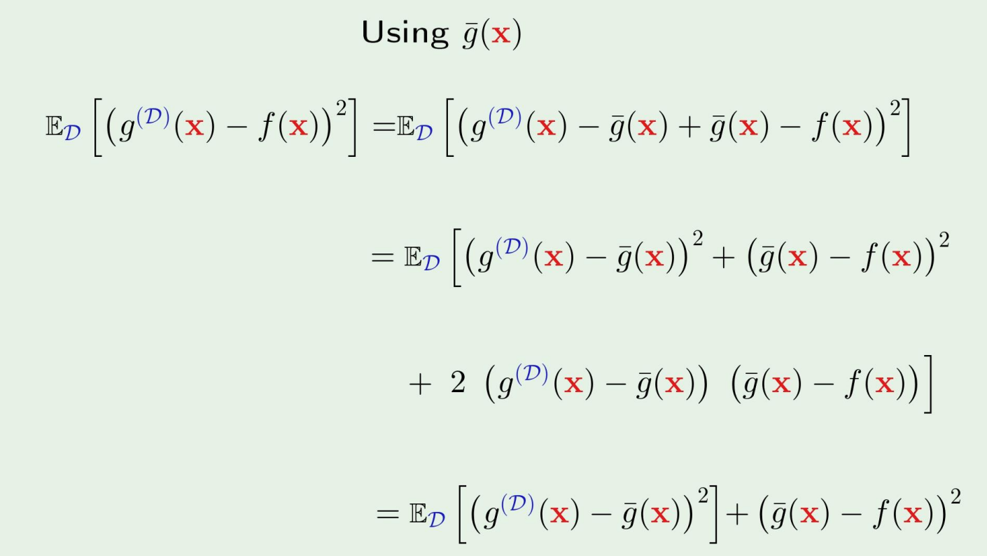
그렇다면 이제, ED[g(D)(x)−f(x)2]를 살펴보자.
The average hypothesis
ED[g(D)(x)−f(x)2]를 evaluate하기 위해 새로운 변수를 하나 정하자.
average hypothesis gˉ(x):
gˉ(x)=ED[g(D)(x)]
gˉ(x)≈K1k=1∑Kg(Dk)(x)
Bias and variance
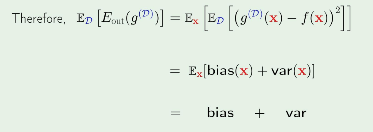
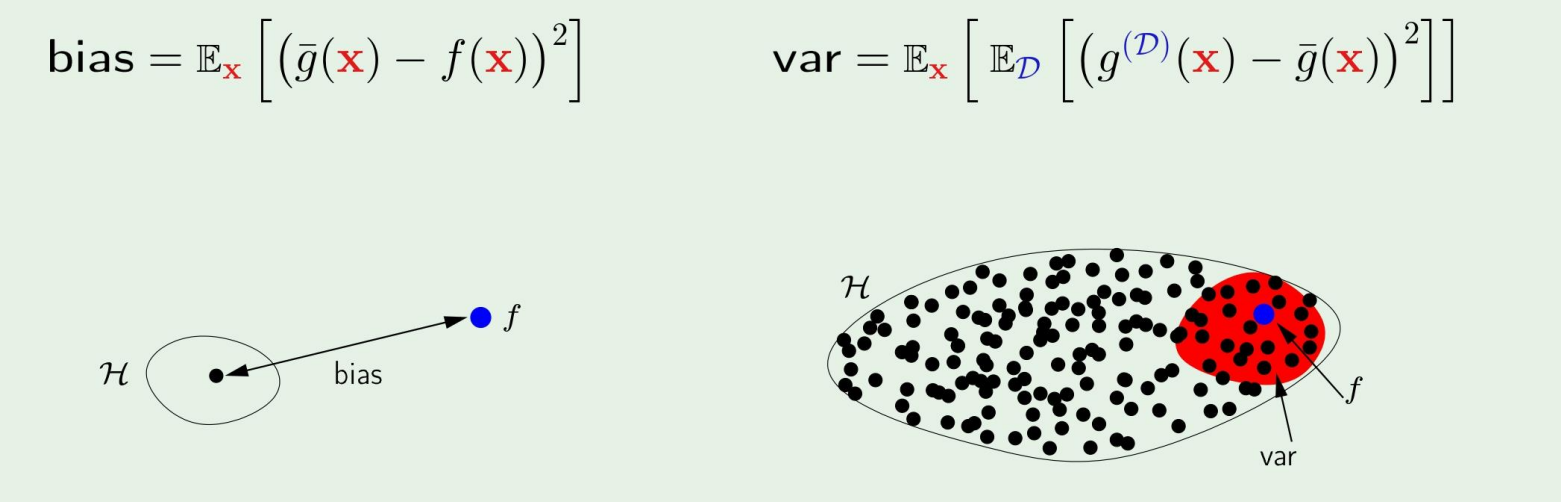
ED[g(D)(x)−f(x)2]=var(x)ED[(g(D)(x)−gˉ(x))2]+bias (x)(gˉ(x)−f(x))2
그렇다면, 다음과 같은 식이 되어 bias와 var에 dependent하게 된다.
bias와 var의 예시를 그림으로 들자면,
왜 tradeoff 문제라고 불릴까?
우리가 set of hypothesis를 크게 만들면 bias가 좀 크더라도 set을 작게 만드는것에 비해 작아질것이다. 그러나 이 경우의 variance가 증가한다.
반대로, variance를 작게 만든다면, bias가 증가한다.
따라서 이 둘을 적절히 조절해야 한다.
한가지 예제를 살펴보자
Example: sine target
f:[−1,1]→Rf(x)=sin(πx)
이 함수를 target function이라 생각하고, 오직 2개의 training example이 있다고 생각하자.
Two model used for learning
H0:H1:h(x)=bh(x)=ax+b
이 경우에 어떤 hypothesis가 더 좋을까?
만약 우리가 target function을 안다면,
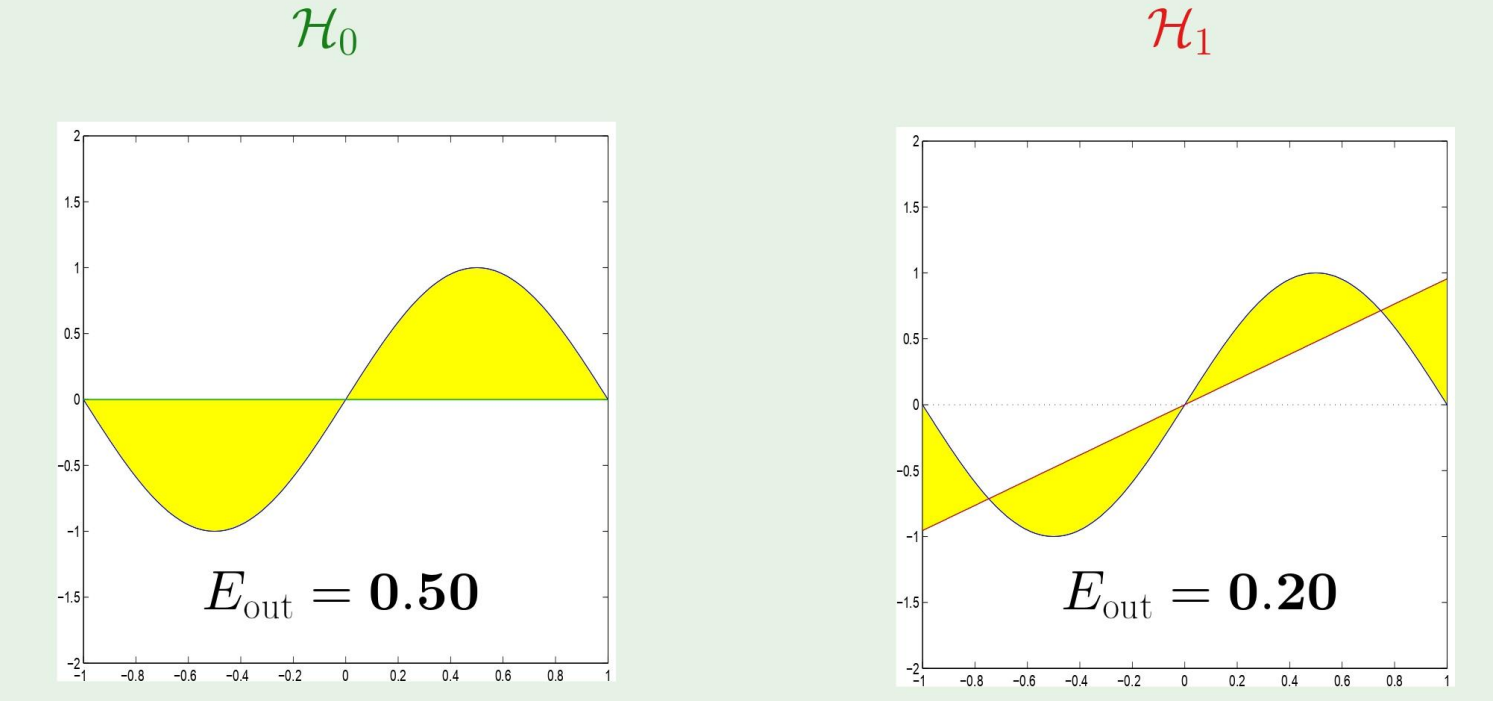
당연히 Eout가 낮은 H1이 더 좋다고 할것이다.
그러나, 우리는 target function을 모르기 때문에, bias variance trade off를 통해 더 나은 h를 찾아야 한다.
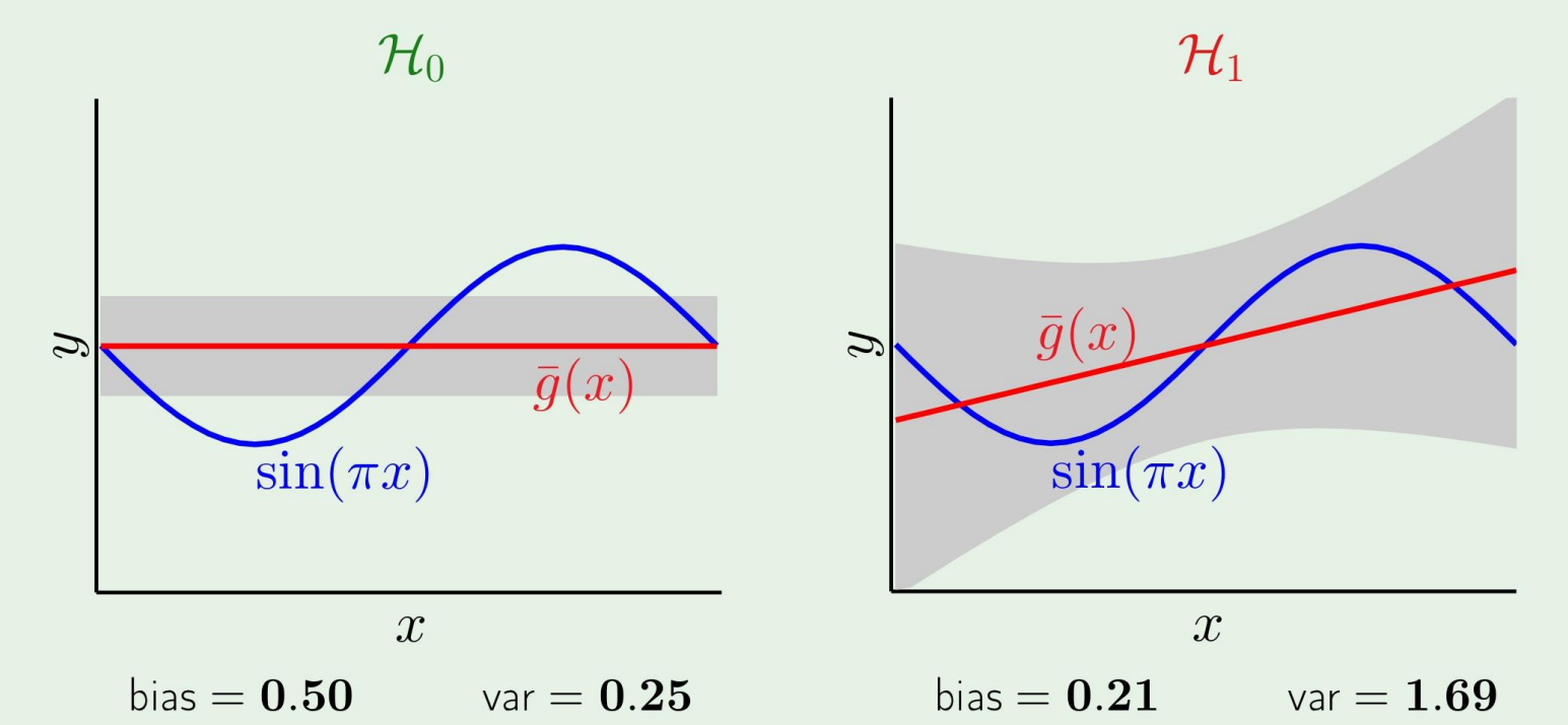
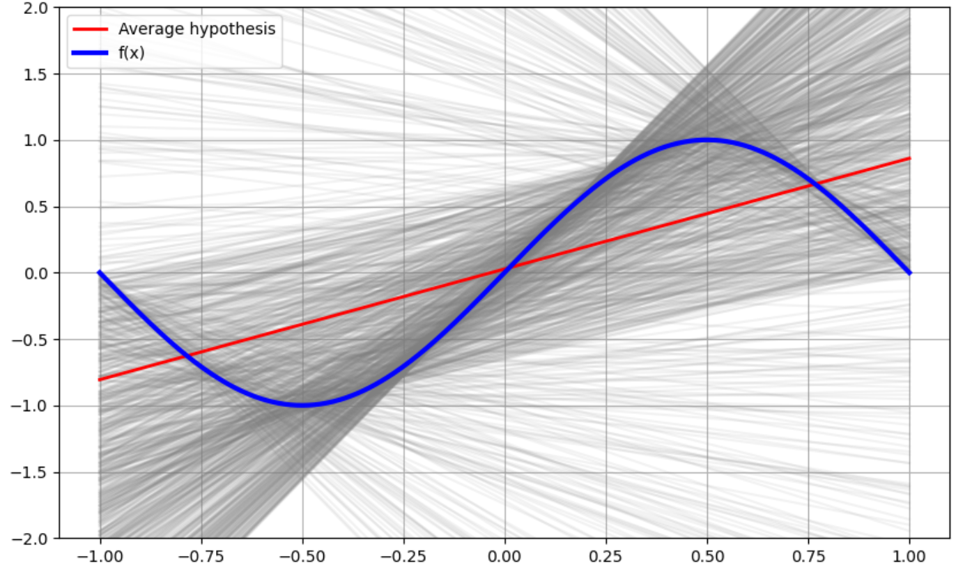
결과를 보면, 아까의 식에서 본것처럼 bias와 variance를 더한것이 우리의 average였으므로, 이 경우에는 H0가 더 좋은 h라 할수있다!
즉, model complexity는 우리가 알수없는 target function에 집중하는것이 아닌, 우리가 실제로 얻은 data에 맞춰야 한다!!
위 과정을 구현해놓았으니 궁금하신분들은 이미지를 누르시면 구현 코드를 확인하실 수 있습니다.
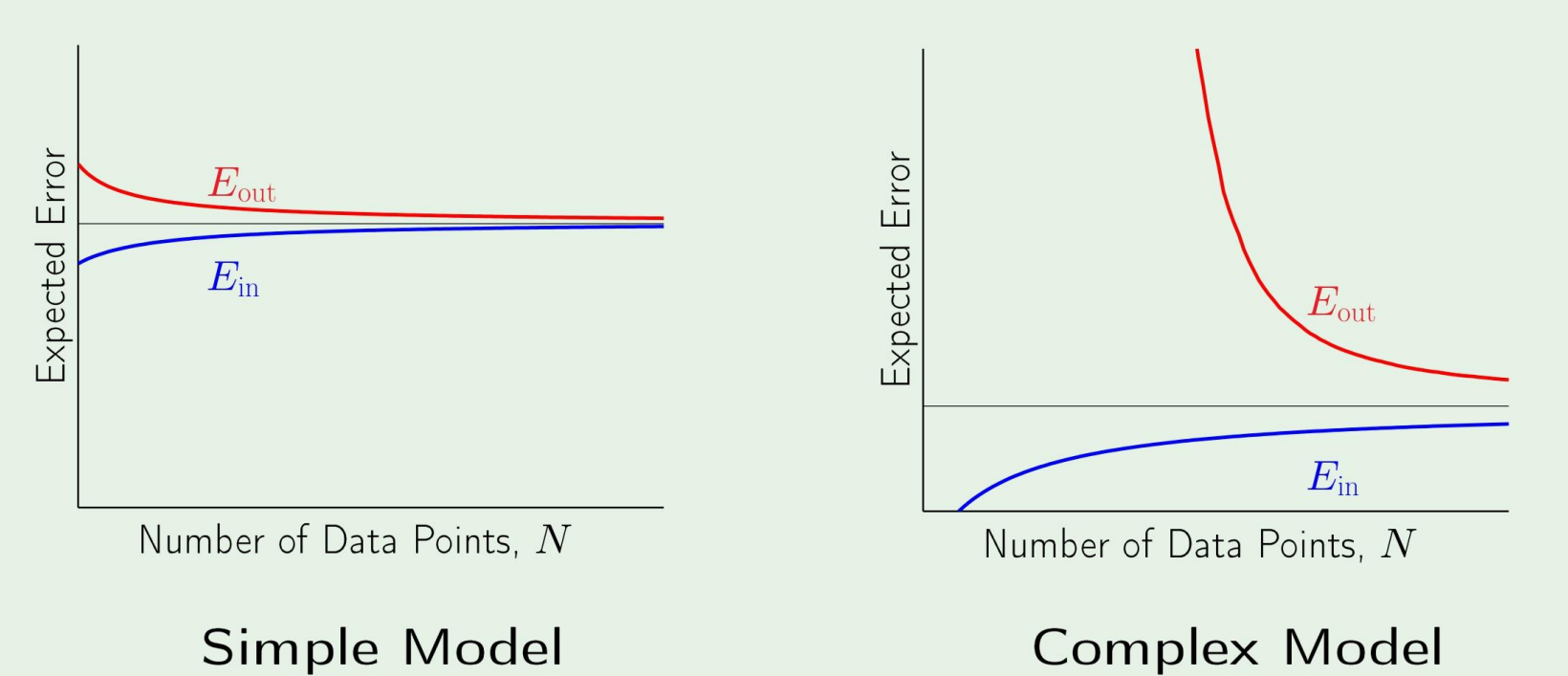
이번엔 sample의 갯수 N이 증가할수록, Ein,Eout이 어떻게 될지 예측해보겠다.
일반적으로, simple model과 complex model에 대한 error는 다음과 같다.
VC analysis vs bias-variance analysis
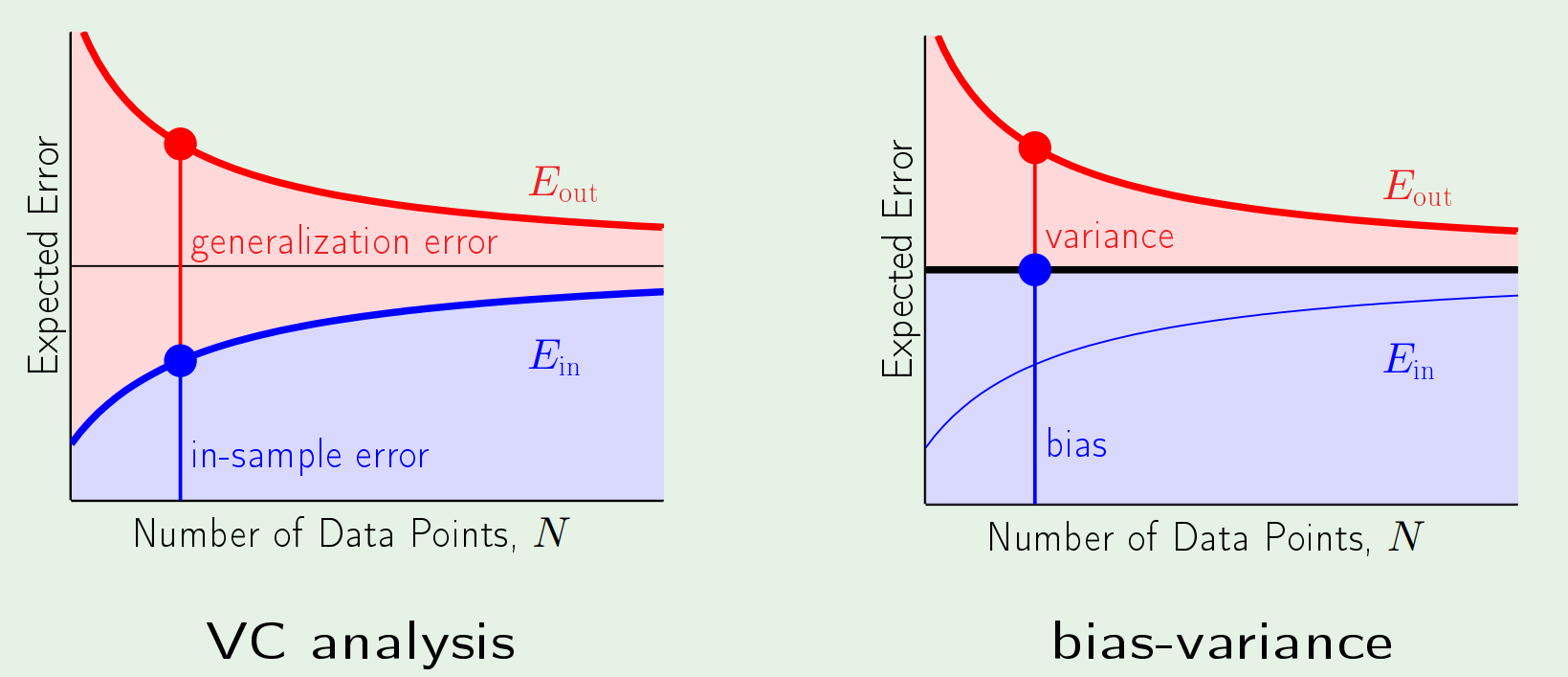
VC analysis에서는 작은 number의 sample에 대해서는 쓸수없다.
