Error and Noise

김민재·2024년 6월 2일

ML

목록 보기

8/17

저번 포스팅에서는 Linear model에 대해 다루었다.
마지막에 Nonlinear transformation에 대해 보았는데, 이번 챕터에서도 계속 보겠다.

Nonlinear transformation (continued)

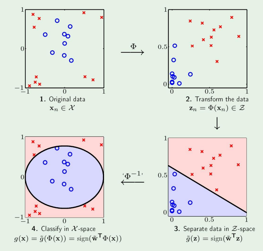
여기서처럼 Inverse mapping을 하면 왜 다시 원래의 boundary로 돌아올까?

선형대수의 Similarity Transformation과 비슷하다.
여기서 결국 data에 대해 mapping을 하는것이고, $w$ 에 대해 하는것이 아니기 때문에 원래 공간으로 hypothesis를 옮겨오면 원래 공간에서 boundary를 나타내게 된다.

식으로 이걸 간단히 확인해보자

\begin{aligned} \mathbf{x} = (x_0, x_1, \cdots,x_d) &\overset{\Phi }{\rightarrow} \mathbf{z} = (z_0, z_1, \cdots, z_{\overset{\sim}{d}})\\ \mathbf{x}_1,\mathbf{x}_2,\cdots,\mathbf{x}_N &\overset{\Phi }{\rightarrow} \mathbf{z}_1,\mathbf{z}_2, \cdots,\mathbf{z}_N\\ y_1,y_2,\cdots,y_N &\overset{\Phi }{\rightarrow} y_1,y_2,\cdots,y_N\\ \end{aligned}

이렇게 label은 바뀌지 않고, $w$ 에 대한 식이므로 원래의 결과로 돌아올 수 있다.

Error measure

지금껏 우리가 찾은 hypothesis와 target function사이의 관계를 모두

h \approx f

로 표기하였다. 이는 당연하게도, 정확한 target을 찾을수없고, 따라서 자연스럽게 error가 생긴다. ML의 목적이 hypothesis를 찾는것도 있지만, 이 error을 줄이는 목표를 잊으면 안된다!

이제 이 error는 $h$ 와 $f$ 에 대한 함수이므로

E(h,f)

로 표기하고, $e(h(x),f(x))$ 로 바꾸는게 가능하다.
ex)

square error : $e(h(x),f(x)) = (h(x) - f(x))^2$
Binary error : $e(h(x),f(x)) = [[h(x)\neq f(x)]]$

From pointwise to overall

그렇다면 이제 $E_{\text{in}}(h,f)$ 와 $E_{\text{out}}(h,f)$ 는 다음처럼 나타낼 수 있다.

In-sample error:

E_{\text{in}}(h) = \frac{1}{N}\sum_{{\color{Red} n}=1}^N e(h(\mathbf{x}_{\color{Red} n}), f(\mathbf{x}_{\color{Red} n}))

Out-of-sample error:

E_{\text{out}}(h) = \mathbb{E}_{\color{Red} n}\left [ e(h({\color{Red} \mathbf{x}}), f({\color{Red} \mathbf{x}})) \right ]

How to choose the error measure

교재에 있는 예제를 그대로 살펴보겠다.

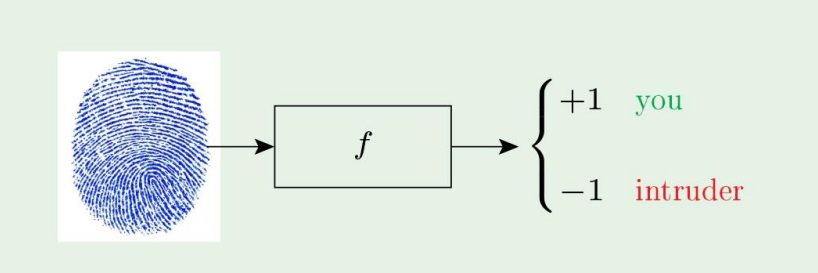
한 지문 인식기를 만들었다고 하자.
그랬을때 confusion matrix는 다음처럼 나타날 것이다.

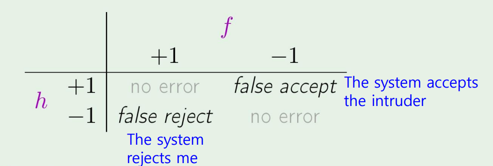
이제 이 지문인식기를 슈퍼마켓과 CIA 두 경우에서 쓰이는 경우를 생각해보자.
슈퍼마켓에서는 피해가 그렇게 크지 않아 error measure를 다음처럼 설정한다 하면,

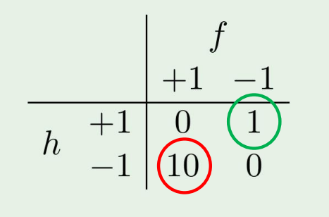
만약 CIA의 경우에는 false accept의 경우에 아주 큰 피해를 가져오므로

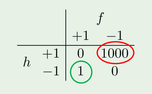
이렇게 크게 설정할수있다.

The error measure should be specified by the user

Noisy target

The target function is not always a function

target function은 우리가 수학적으로 생각하는 그런 함수가 아닐수있다!

따라서...

Target 'distribution'

$y = f(x)$ 대신에, 우리는 target distribution $P(y|x)$ 를 사용하자.
$(x,y)$ 는 이제 joint distribution $P(x)P(y|x)$ 로 표현되고,

Noisy target = deterministic target $f(x) = \mathbb{E}(y|x)$ + noise $y - f(x)$

Deterministic target is a special case of noisy target

P(y|x) \text{ is zero except for }y = f(\mathbf{x})

이제 좀더 Learning 이라는것에 집중해보자.
우리가 호패딩형님에 의해서 Learning is feasible하다는 것을 알았다.

E_{\text{out}}(g) \approx E_{\text{in}}(g)

이것은 learning이 아니다.
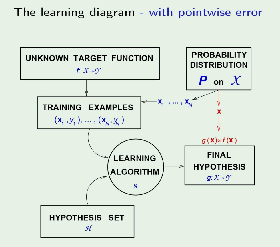
우리가 learning을 하려는 것은, $E_{\text{out}}(g) \approx 0$ 을 찾는것이다.

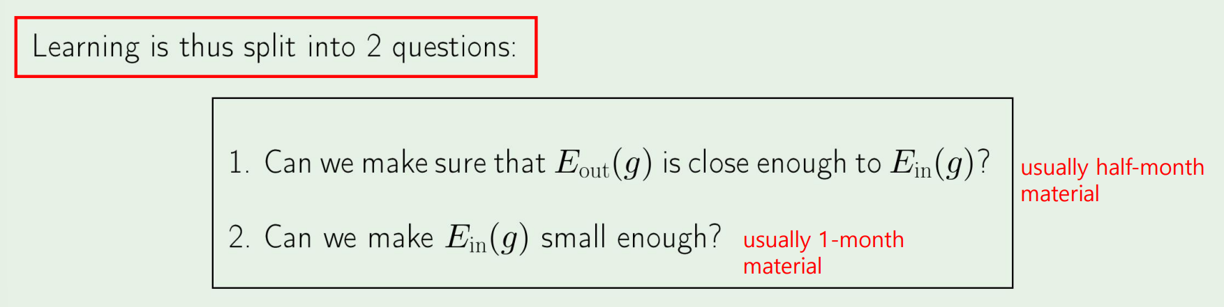
Learning이란, 위 그림의 2가지 문제를 푸는것이다.

더 깊게 learning에 집중하기 전에 다음의 tradeoff 문제를 살펴보자.
결국 우리는 model complexity를 결정하며 문제를 어떻게 풀어야 할지 정해야하는데,

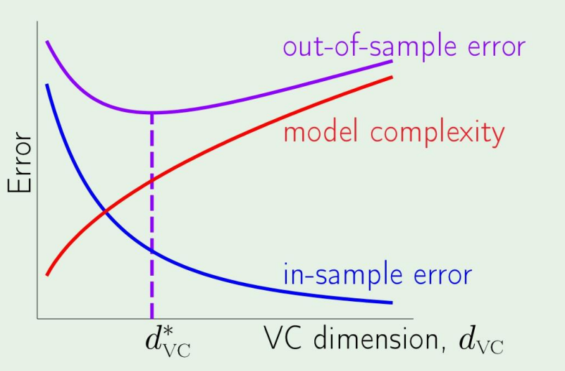
그림에서 볼수있듯이
Model complexity가 올라가면 $E_{\text{in}}$ 는 낮아지지만, $E_{\text{out}} - E_{\text{in}}$ 은 커지게 된다.
근데 이 complexity를 어느정도 정할수있는데, 이는 다음 포스팅에서 살펴보겠다.

김민재

이전 포스트

The Linear Model

다음 포스트