이번 장에서는 Regularization, 그중에서도 curve fitting problem만 간단하게 다뤄보겠다.
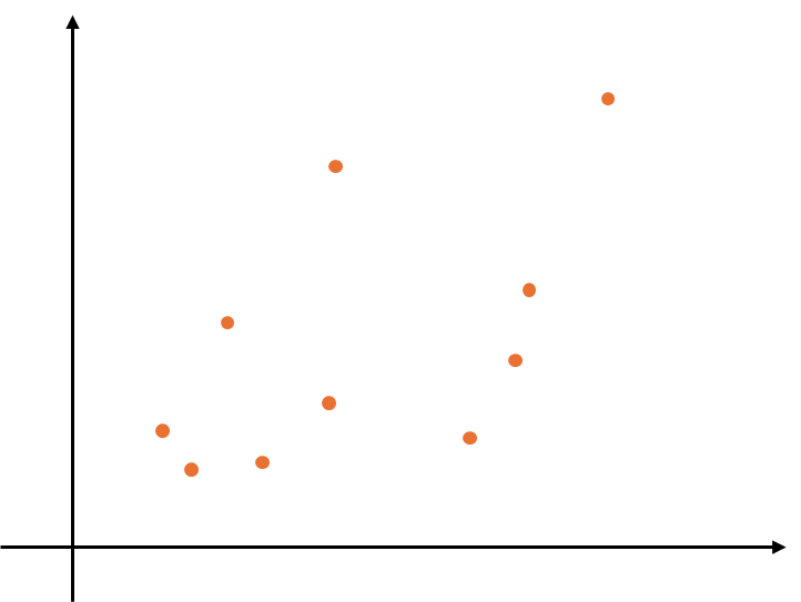
이러한 점들이 존재할때, 과연 몇차원으로 fitting을 해야할지 결정하는 것이다. (polynomial regression)
결론부터 말하면, 내 hypothesis space가 Legendre polynomials로 이루어 진다고 볼 수 있다.
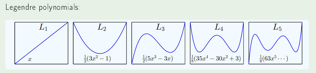
바꿔 말하면, 내가 구하려는 hypothesis, target function을 Legendre polynomials의 sum으로 볼수있다.
HQ:polynomials of order Qz=⎣⎢⎢⎢⎢⎡1L1(x)⋮LQ(x)⎦⎥⎥⎥⎥⎤linear regression in Z spaceH={q=0∑QwqLq(x)}
그러면 우리가 (x1,y1),⋯,(xN,yN) 이라는 점들이 주어졌을때, x를 z로 transform해 (z1,y1)⋯,(zN,yN)로 나타내고,
이것을 이제 최소화 하는 w를 찾아야 하므로,
Minimize Ein(w)=N1n=1∑N(wTzn−yn)2Minimize N1(Zw−y)T(Zw−y)wlin=(ZTZ)−1ZTy
예전에 배웠듯이 normal equation으로 풀수있다.
이제 내가 어떤 curve fitting을 해야 하는데, 10개의 sum으로 나타내야될거 같다고 생각하자 →H10
그런데 여기에 제약조건이 걸리게 된다.
Hard constraint :H2 is constrained version of H10 with wq=0 for q>2
즉 L1,L2를 제외하고는 모두 0으로 만들어 버린다는 뜻이다.
그러나 이렇게 하면 내가 원하는 fitting이 안될수도 있으므로, soft한 constraint를 부여한다.
Softer version :q=0∑Qwq2≤C "soft-order" constraint
즉 L1,L2까지는 원래의 식을 그대로 쓰고, L3부터는 C보다 작은 값으로 맞춰준다는 것이다.
이렇게 구속조건을 걸어준 뒤에, 다시 minimize를 하면,
N1(Zw−y)T(Zw−y)
subject to:wTw≤C
아까와 같은 식에, wTw≤C 구속조건만 더해졌다.
이렇게 나온 w를, wlin 대신에 wreg 라고 하자.
Solving for wreg
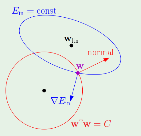
파란색원이 구속조건이 없는 상태이고, 그 위에 빨간색 원이 구속조건이다.
그렇다면 이제 식을 보자
∇Ein(wreg)∝−wreg=−2Nλwreg
∇Ein(wreg)+2Nλwreg=0
Minimize Ein(w)+NλwTw
여기서 λ는 우리가 SVM에 Augmented target function의 그 λ 이다.
Solution
Minimize Eaug(w)=Ein(w)+NλwTw=N1((Zw−y)T(Zw−y)+λwTw)
∇Eaug(w)=0⟹ZT(Zw−y)+λw=0
이 식을 풀면 우리는 augmented target function에 대한 minimize를 할 수 있다.
wregwlin=(ZTZ+λI)−1ZTy=(ZTZ)−1ZTy
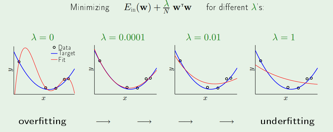
그림을 살펴보면 λ=0일때는 no regulization을 한다는 의미이다.
그리고 그림의 식에 있는 wTw는 우리가 알고있는 Ridge Regularlization이다.
