IMDb 데이터셋
- 50000개의 영화리뷰 텍스트 (영문)
- 긍정은 1, 부정은 0으로 라벨링 되어있음
1. 문장 길이 동일하게 세팅
import tensorflow as tf
from tensorflow import keras
import numpy as np

print(tf.__version__)
imdb = keras.datasets.imdb

(x_train, y_train), (x_test, y_test) = imdb.load_data(num_words = 10000)
print("훈련 샘플 개수: {}, 테스트 개수: {}".format(len(x_train), len(x_test)))
2.6.0
훈련 샘플 개수: 25000, 테스트 개수: 25000
imdb.load_data()호출 시 단어사전에 등재할 단어의 개수(num_words)를 10000으로 지정하면, 그 개수만큼의 word_to_index 딕셔너리까지 생성된 형태로 데이터셋이 생성됨
print(x_train[0])
print('label', y_train[0])

print('첫번째 리뷰 문장 길이: ', len(x_train[0]))
print('두번째 리뷰 문장 길이: ', len(x_train[1]))
[1, 14, 22, 16, 43, 530, 973, 1622, 1385, 65, 458, 4468, 66, 3941, 4, 173, 36, 256, 5, 25, 100, 43, 838, 112, 50, 670, 2, 9, 35, 480, 284, 5, 150, 4, 172, 112, 167, 2, 336, 385, 39, 4, 172, 4536, 1111, 17, 546, 38, 13, 447, 4, 192, 50, 16, 6, 147, 2025, 19, 14, 22, 4, 1920, 4613, 469, 4, 22, 71, 87, 12, 16, 43, 530, 38, 76, 15, 13, 1247, 4, 22, 17, 515, 17, 12, 16, 626, 18, 2, 5, 62, 386, 12, 8, 316, 8, 106, 5, 4, 2223, 5244, 16, 480, 66, 3785, 33, 4, 130, 12, 16, 38, 619, 5, 25, 124, 51, 36, 135, 48, 25, 1415, 33, 6, 22, 12, 215, 28, 77, 52, 5, 14, 407, 16, 82, 2, 8, 4, 107, 117, 5952, 15, 256, 4, 2, 7, 3766, 5, 723, 36, 71, 43, 530, 476, 26, 400, 317, 46, 7, 4, 2, 1029, 13, 104, 88, 4, 381, 15, 297, 98, 32, 2071, 56, 26, 141, 6, 194, 7486, 18, 4, 226, 22, 21, 134, 476, 26, 480, 5, 144, 30, 5535, 18, 51, 36, 28, 224, 92, 25, 104, 4, 226, 65, 16, 38, 1334, 88, 12, 16, 283, 5, 16, 4472, 113, 103, 32, 15, 16, 5345, 19, 178, 32]
label 1
첫번째 리뷰 문장 길이: 218
두번째 리뷰 문장 길이: 189- 위의 결과를 통해 encoding된 텍스트를 다운받았음을 확인할 수 있음
# Always Remind - encoding을 했으면 다시 되돌리는 decoding 함수가 필요함

word_to_index = imdb.get_word_index()
index_to_word = {index:word for word, index in word_to_index.items()}
print(index_to_word[1])
print(word_to_index['the'])
the
1- word_to_index 데이터가 어떻게 되어있는지 확인하기 위해 dict to DF 진행
# list(sorted(word_to_index.items(), key = lambda item : item[0]))| key | value | |
|---|---|---|
| 0 | fawn | 34701 |
| 1 | tsukino | 52006 |
| 2 | nunnery | 52007 |
| 3 | sonja | 16816 |
| 4 | vani | 63951 |
| ... | ... | ... |
| 88579 | voorhees' | 88583 |
| 88580 | 35mm | 16815 |
| 88581 | 'l' | 88584 |
| 88582 | paget | 18509 |
| 88583 | expands | 20597 |
88584 rows × 2 columns
# Tip
# Dictionary to Dataframe 다양한 모양
import pandas as pd

# 방법1
method1 = pd.DataFrame(list(word_to_index.items()), columns = ['word', 'index'])
# list(sorted(word_to_index.items(), key = lambda item : item[0])) # key 기준으로 list sorted 진행

# 방법2
method2 = pd.DataFrame([word_to_index])

# 방법3 : key를 행으로 사용하고 열 이름을 변경하기 위해 orient = 'index' 설정
method3 = pd.DataFrame.from_dict(word_to_index, orient = 'index').rename(columns = {0: 'index'})method1.sort_values(by = 'index', ascending=False)| word | index | |
|---|---|---|
| 88581 | 'l' | 88584 |
| 88579 | voorhees' | 88583 |
| 88576 | artbox | 88582 |
| 88574 | copywrite | 88581 |
| 88571 | pipe's | 88580 |
| ... | ... | ... |
| 67377 | to | 5 |
| 20340 | of | 4 |
| 37291 | a | 3 |
| 64304 | and | 2 |
| 58318 | the | 1 |
88584 rows × 2 columns
- IMDb 데이터셋의 텍스트 인코딩을 위한 word_to_index, index_to_word는 아래와 같이 보정되어야함
# 아래의 index 추가를 위해 약간의 수정을 진행함
word_to_index = {k:(v+3) for k,v in word_to_index.items()}

word_to_index["<PAD>"] = 0
word_to_index["<BOS>"] = 1
word_to_index["<UNK>"] = 2  # unknown
word_to_index["<UNUSED>"] = 3

index_to_word[0] = "<PAD>"
index_to_word[1] = "<BOS>"
index_to_word[2] = "<UNK>"
index_to_word[3] = "<UNUSED>"

index_to_word = {index:word for word, index in word_to_index.items()}

print(index_to_word[1])
print(word_to_index['the'])
print(index_to_word[4]) <BOS>
4
theprint(get_decoded_sentence(x_train[0], index_to_word))
print('라벨: ', y_train[0]) # 1번째 리뷰데이터의 라벨this film was just brilliant casting location scenery story direction everyone's really suited the part they played and you could just imagine being there robert <UNK> is an amazing actor and now the same being director <UNK> father came from the same scottish island as myself so i loved the fact there was a real connection with this film the witty remarks throughout the film were great it was just brilliant so much that i bought the film as soon as it was released for <UNK> and would recommend it to everyone to watch and the fly fishing was amazing really cried at the end it was so sad and you know what they say if you cry at a film it must have been good and this definitely was also <UNK> to the two little boy's that played the <UNK> of norman and paul they were just brilliant children are often left out of the <UNK> list i think because the stars that play them all grown up are such a big profile for the whole film but these children are amazing and should be praised for what they have done don't you think the whole story was so lovely because it was true and was someone's life after all that was shared with us all
라벨: 1- pad_sequences를 통해 데이터셋 상의 문장의 길이를 통일하는 것을 꼭 기억
- 문장 최대 길이 maxlen의 값 설정도 전체 모델 성능에 영향을 미치게 됨
- maxlen의 적절한 값을 찾기 위해서는 전체 데이터셋의 분포를 확인해 보는 것이 좋음
# 텍스트 데이터 문장길이의 리스트를 생성
total_data_text = list(x_train) + list(x_test)
# print(len(total_data_text)) # 전체 data 50000개 확인
# len(total_data_text) # num of rows
# len(total_data_text[0]) # num of columns

# 한 문장당 길이를 확인
num_tokens = [len(tokens) for tokens in total_data_text]
# print(num_tokens)
num_tokens = np.array(num_tokens)

# 문장길이의 평균값, 최대값, 표준편차를 계산
print('문장길이 평균 : ', np.mean(num_tokens))
print('문장길이 최대 : ', np.max(num_tokens))
print('문장길이 표준편차 : ', np.std(num_tokens))

# 최대길이를 (평균 + 2*표준편차)로 설정
max_tokens = np.mean(num_tokens) + 2 * np.std(num_tokens)
maxlen = int(max_tokens)

print('pad_sequences maxlen : ', maxlen)
print('전체 문장의 {}%가 maxlen 설정값 이내에 포함. '.format(np.sum(num_tokens < max_tokens) / len(num_tokens)))
# num_tokens < max_tokens 은 True False로 값 나옴
문장길이 평균 : 234.75892
문장길이 최대 : 2494
문장길이 표준편차 : 172.91149458735703
pad_sequences maxlen : 580
전체 문장의 0.94536%가 maxlen 설정값 이내에 포함.num_tokens < max_tokensarray([ True, True, True, ..., True, True, True])2 Padding | Post & Pre
- Post Padding vs Pre Padding에 의해 딥러닝 성능이 다르게 나옴
x_train = keras.preprocessing.sequence.pad_sequences(x_train, value = word_to_index['<PAD>'],
                                                    padding = 'post', maxlen = maxlen)

x_test = keras.preprocessing.sequence.pad_sequences(x_test,
                                                    value=word_to_index["<PAD>"],
                                                    padding='post',
                                                    maxlen=maxlen)

print(x_train.shape, x_test.shape)
(25000, 580) (25000, 580)- RNN은 입력데이터가 순차적으로 처리되어, 가장 마지막 입력이 최종 state 값에 가장 영향을 많이 미침
- 그러므로 마지막 입력이 무의미한 padding으로 채워지는 것은 비효율적
- 따라서 'pre'가 훨씬 유리하며, 10% 이상의 테스트 성능 차이를 보이게 됨
# dataset _ validation set 만들기
# 여기서는 25000 중 10000건을 vali로 사용하고자 함
x_val = x_train[:10000]
y_val = y_train[:10000]

partial_x_train = x_train[10000:]
partial_y_train = y_train[10000:]

print(partial_x_train.shape)
print(partial_y_train.shape)
(15000, 580)
(15000,)3. 딥러닝 모델 설계와 훈련
3-1. Model_1 생성
# Model_1 생성

vocab_size = 10000 # word 사전의 크기. 단어 10000개
word_vector_dim = 16

model_1 = keras.Sequential(name = 'model1')

# shape = (None,)은 모양이 알려지지 않은 수치를 표시할 때 사용됨
# mask_zero = True : padding 부분 인지시켜주기 위해 진행
model_1.add(keras.layers.Embedding(vocab_size, word_vector_dim, input_shape = (None,),
                                mask_zero = True, name = 'word_embedding'))
model_1.add(keras.layers.LSTM(units = 32)) # units는 출력 차원, activation은 default로 tanh, dropout도 존재
model_1.add(keras.layers.Dense(8, activation='relu'))
model_1.add(keras.layers.Dense(1, activation='sigmoid'))  # 최종 출력은 긍정/부정을 나타내는 1dim

model_1.summary()

# numpy 1.20v 에서 안되서 colab에서 실행시킴 (1.19v)
Model: "model1"
_________________________________________________________________
Layer (type) Output Shape Param #
=================================================================
word_embedding (Embedding) (None, None, 16) 160000
_________________________________________________________________
lstm_4 (LSTM) (None, 32) 6272
_________________________________________________________________
dense_16 (Dense) (None, 8) 264
_________________________________________________________________
dense_17 (Dense) (None, 1) 9
=================================================================
Total params: 166,545
Trainable params: 166,545
Non-trainable params: 0
_________________________________________________________________3-2. Model_2 생성
# Model_2 생성

vocab_size = 10000
word_vector_dim = 16

model_2 = keras.Sequential(name = 'model2')
model_2.add(keras.layers.Embedding(vocab_size, word_vector_dim,
                                input_shape = (None, ), mask_zero = True))
model_2.add(keras.layers.Conv1D(32, 16, activation = 'relu'))
model_2.add(keras.layers.MaxPooling1D(4))
model_2.add(keras.layers.Conv1D(32, 16, activation='relu'))
model_2.add(keras.layers.GlobalMaxPool1D())
model_2.add(keras.layers.Dense(10, activation='relu'))
model_2.add(keras.layers.Dense(1, activation = 'sigmoid'))

model_2.summary()
Model: "model2"
_________________________________________________________________
Layer (type) Output Shape Param #
=================================================================
embedding_7 (Embedding) (None, None, 16) 160000
_________________________________________________________________
conv1d_8 (Conv1D) (None, None, 32) 8224
_________________________________________________________________
max_pooling1d_4 (MaxPooling1 (None, None, 32) 0
_________________________________________________________________
conv1d_9 (Conv1D) (None, None, 32) 16416
_________________________________________________________________
global_max_pooling1d_5 (Glob (None, 32) 0
_________________________________________________________________
dense_18 (Dense) (None, 10) 330
_________________________________________________________________
dense_19 (Dense) (None, 1) 11
=================================================================
Total params: 184,981
Trainable params: 184,981
Non-trainable params: 0
_________________________________________________________________4. Model 학습
4-1. Model_1 학습
# model1 사용

# 긍정 부정만 확인하는 거라서 loss를 binary crossentropy로 진행
model_1.compile(optimizer = 'adam', loss = 'binary_crossentropy',
              metrics = ['accuracy'])

epochs = 20

history_1 = model_1.fit(partial_x_train, partial_y_train, epochs = epochs,
                        batch_size = 512, validation_data = (x_val, y_val),
                        verbose = 1)
Epoch 1/20
30/30 [==============================] - 50s 2s/step - loss: 0.6923 - accuracy: 0.5587 - val_loss: 0.6890 - val_accuracy: 0.5880
Epoch 2/20
30/30 [==============================] - 44s 1s/step - loss: 0.6468 - accuracy: 0.7024 - val_loss: 0.6610 - val_accuracy: 0.6041
Epoch 3/20
30/30 [==============================] - 44s 1s/step - loss: 0.5661 - accuracy: 0.7670 - val_loss: 0.4950 - val_accuracy: 0.7951
Epoch 4/20
30/30 [==============================] - 44s 1s/step - loss: 0.3879 - accuracy: 0.8648 - val_loss: 0.3862 - val_accuracy: 0.8523
Epoch 5/20
30/30 [==============================] - 44s 1s/step - loss: 0.2868 - accuracy: 0.9005 - val_loss: 0.3129 - val_accuracy: 0.8794
Epoch 6/20
30/30 [==============================] - 44s 1s/step - loss: 0.2194 - accuracy: 0.9269 - val_loss: 0.3038 - val_accuracy: 0.8814
Epoch 7/20
30/30 [==============================] - 45s 2s/step - loss: 0.1713 - accuracy: 0.9447 - val_loss: 0.2857 - val_accuracy: 0.8865
Epoch 8/20
30/30 [==============================] - 45s 1s/step - loss: 0.1531 - accuracy: 0.9517 - val_loss: 0.3015 - val_accuracy: 0.8844
Epoch 9/20
30/30 [==============================] - 46s 2s/step - loss: 0.1255 - accuracy: 0.9631 - val_loss: 0.3047 - val_accuracy: 0.8808
Epoch 10/20
30/30 [==============================] - 46s 2s/step - loss: 0.1070 - accuracy: 0.9705 - val_loss: 0.3675 - val_accuracy: 0.8776
Epoch 11/20
30/30 [==============================] - 46s 2s/step - loss: 0.0825 - accuracy: 0.9795 - val_loss: 0.3525 - val_accuracy: 0.8817
Epoch 12/20
30/30 [==============================] - 46s 2s/step - loss: 0.0662 - accuracy: 0.9851 - val_loss: 0.3836 - val_accuracy: 0.8801
Epoch 13/20
30/30 [==============================] - 46s 2s/step - loss: 0.0534 - accuracy: 0.9889 - val_loss: 0.4144 - val_accuracy: 0.8732
Epoch 14/20
30/30 [==============================] - 46s 2s/step - loss: 0.0477 - accuracy: 0.9909 - val_loss: 0.4640 - val_accuracy: 0.8718
Epoch 15/20
30/30 [==============================] - 45s 2s/step - loss: 0.0410 - accuracy: 0.9925 - val_loss: 0.4845 - val_accuracy: 0.8703
Epoch 16/20
30/30 [==============================] - 45s 2s/step - loss: 0.0361 - accuracy: 0.9933 - val_loss: 0.5271 - val_accuracy: 0.8672
Epoch 17/20
30/30 [==============================] - 45s 2s/step - loss: 0.0329 - accuracy: 0.9940 - val_loss: 0.5167 - val_accuracy: 0.8680
Epoch 18/20
30/30 [==============================] - 46s 2s/step - loss: 0.0290 - accuracy: 0.9953 - val_loss: 0.5918 - val_accuracy: 0.8601
Epoch 19/20
30/30 [==============================] - 45s 2s/step - loss: 0.0634 - accuracy: 0.9813 - val_loss: 0.4286 - val_accuracy: 0.8488
Epoch 20/20
30/30 [==============================] - 45s 2s/step - loss: 0.0621 - accuracy: 0.9811 - val_loss: 0.5331 - val_accuracy: 0.8656
result_1 = model_1.evaluate(x_test, y_test, verbose = 2)
print(result_1)782/782 - 48s - loss: 0.5897 - accuracy: 0.8451
[0.5897064208984375, 0.8450800180435181]4-2. Model_2 학습
# model2 사용

model_2.compile(optimizer = 'adam', loss = 'binary_crossentropy',
              metrics = ['accuracy'])
epochs = 20

history_2 = model_2.fit(partial_x_train, partial_y_train, epochs = epochs,
                        batch_size = 512, validation_data = (x_val, y_val),
                        verbose = 1)

from keras.callbacks import EarlyStopping
early_stopping = EarlyStopping(monitor='loss', patience=100, mode='auto')

# # 이거 사용하면 중간에 멈춰. 최적일때
# model_2.fit(x_test, y_test, epochs=1, batch_size=1, verbose=2, callbacks=[early_stopping])
Epoch 1/20
30/30 [==============================] - 29s 947ms/step - loss: 0.6930 - accuracy: 0.5056 - val_loss: 0.6924 - val_accuracy: 0.5112
Epoch 2/20
30/30 [==============================] - 28s 933ms/step - loss: 0.6765 - accuracy: 0.6681 - val_loss: 0.6112 - val_accuracy: 0.7532
Epoch 3/20
30/30 [==============================] - 28s 936ms/step - loss: 0.4227 - accuracy: 0.8275 - val_loss: 0.3347 - val_accuracy: 0.8557
Epoch 4/20
30/30 [==============================] - 28s 935ms/step - loss: 0.2392 - accuracy: 0.9036 - val_loss: 0.3100 - val_accuracy: 0.8697
Epoch 5/20
30/30 [==============================] - 28s 936ms/step - loss: 0.1602 - accuracy: 0.9435 - val_loss: 0.3168 - val_accuracy: 0.8746
Epoch 6/20
30/30 [==============================] - 28s 934ms/step - loss: 0.1076 - accuracy: 0.9653 - val_loss: 0.3600 - val_accuracy: 0.8694
Epoch 7/20
30/30 [==============================] - 28s 934ms/step - loss: 0.0699 - accuracy: 0.9818 - val_loss: 0.4195 - val_accuracy: 0.8652
Epoch 8/20
30/30 [==============================] - 28s 939ms/step - loss: 0.0437 - accuracy: 0.9899 - val_loss: 0.5086 - val_accuracy: 0.8588
Epoch 9/20
30/30 [==============================] - 28s 932ms/step - loss: 0.0270 - accuracy: 0.9961 - val_loss: 0.5540 - val_accuracy: 0.8585
Epoch 10/20
30/30 [==============================] - 28s 929ms/step - loss: 0.0158 - accuracy: 0.9979 - val_loss: 0.6197 - val_accuracy: 0.8542
Epoch 11/20
30/30 [==============================] - 28s 933ms/step - loss: 0.0107 - accuracy: 0.9992 - val_loss: 0.6848 - val_accuracy: 0.8556
Epoch 12/20
30/30 [==============================] - 28s 934ms/step - loss: 0.0066 - accuracy: 0.9995 - val_loss: 0.7504 - val_accuracy: 0.8556
Epoch 13/20
30/30 [==============================] - 28s 931ms/step - loss: 0.0038 - accuracy: 0.9996 - val_loss: 0.7932 - val_accuracy: 0.8562
Epoch 14/20
30/30 [==============================] - 28s 931ms/step - loss: 0.0021 - accuracy: 0.9998 - val_loss: 0.8313 - val_accuracy: 0.8555
Epoch 15/20
30/30 [==============================] - 28s 929ms/step - loss: 0.0013 - accuracy: 0.9999 - val_loss: 0.8680 - val_accuracy: 0.8551
Epoch 16/20
30/30 [==============================] - 28s 932ms/step - loss: 0.0010 - accuracy: 0.9999 - val_loss: 0.8960 - val_accuracy: 0.8555
Epoch 17/20
30/30 [==============================] - 28s 929ms/step - loss: 8.4985e-04 - accuracy: 0.9999 - val_loss: 0.9178 - val_accuracy: 0.8559
Epoch 18/20
30/30 [==============================] - 28s 931ms/step - loss: 7.3165e-04 - accuracy: 0.9999 - val_loss: 0.9421 - val_accuracy: 0.8556
Epoch 19/20
30/30 [==============================] - 28s 931ms/step - loss: 6.1983e-04 - accuracy: 0.9999 - val_loss: 0.9628 - val_accuracy: 0.8553
Epoch 20/20
30/30 [==============================] - 28s 943ms/step - loss: 4.8885e-04 - accuracy: 0.9999 - val_loss: 0.9842 - val_accuracy: 0.8541result_2 = model_2.evaluate(x_test, y_test, verbose = 2)
print(result_2)782/782 - 9s - loss: 0.3405 - accuracy: 0.8480
[0.34045761823654175, 0.8479599952697754]비고. Early Stopping
# ## Early stopping을 이용해서 acc max, loss min을 찾아

# model = Sequential()
# # model.add(LSTM(20, activation = 'relu', input_shape=(3,1))) # (None, 3, 1)
# # model.add(LSTM(3)) # (None, 3) -> Value error
# model.add(LSTM(10, activation = 'relu', input_shape=(3,1), return_sequences=True))
# model.add(LSTM(10, activation = 'relu', return_sequences=True)) # (None, 3, 10)을 받는다
# model.add(LSTM(10, activation = 'relu', return_sequences=True))
# model.add(LSTM(10, activation = 'relu', return_sequences=True))
# model.add(LSTM(10, activation = 'relu', return_sequences=True))
# model.add(LSTM(10, activation = 'relu', return_sequences=True))
# model.add(LSTM(10, activation = 'relu', return_sequences=True))
# model.add(LSTM(10, activation = 'relu', return_sequences=True))
# model.add(LSTM(3)) # 마지막은 return_sequence X
# # return_sequence를 쓰면 dimension이 한개 추가 되므로 다음 Dense Layer의 인풋에 3 dim이 들어가게 되므로 안씀
# # LSTM 두개를 엮을 때
# model.add(Dense(5))
# model.add(Dense(1))

# model.summary()

# model.compile(optimizer='adam', loss='mse')

# from keras.callbacks import EarlyStopping
# early_stopping = EarlyStopping(monitor='loss', patience=100, mode='auto')
# model.fit(x, y, epochs=1, batch_size=1, verbose=2, callbacks=[early_stopping])

# x_input = array([25,35,45]) # predict용
# x_input = x_input.reshape((1,3,1))

# yhat = model.predict(x_input)
# print(yhat)

# # LSTM을 2개 이상 많이 엮으면 좋지 않다.


# 출처: https://ebbnflow.tistory.com/135 [Dev Log : 삶은 확률의 구름]
5. Model 저장
5-1. Model 저장
from keras.models import load_model

model_1.save('node_method_model.h5')
model_2.save('other_method_model.h5')
5-2. Graph로 학습 아이디어 얻기
history_dict_1 = history_1.history
print(history_dict_1.keys()) # epoch에 따른 그래프를 그려볼 수 있는 항목들
dict_keys(['loss', 'accuracy', 'val_loss', 'val_accuracy'])history_dict_2 = history_2.history
print(history_dict_2.keys()) # epoch에 따른 그래프를 그려볼 수 있는 항목들dict_keys(['loss', 'accuracy', 'val_loss', 'val_accuracy'])# model_1, history_1 Training and validation Loss
import matplotlib.pyplot as plt
acc1 = history_dict_1['accuracy']
val_acc1 = history_dict_1['val_accuracy']
loss1 = history_dict_1['loss']
val_loss1 = history_dict_1['val_loss']
epochs1 = range(1, len(acc1) + 1)
# "bo"는 "파란색 점"
plt.plot(epochs1, loss1, 'bo', label='Training loss')
# b는 "파란 실선"
plt.plot(epochs1, val_loss1, 'b', label='Validation loss')
plt.title('Training and validation loss')
plt.xlabel('Epochs')
plt.ylabel('Loss')
plt.legend()
plt.show()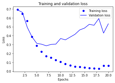
# Training and validation accuracy

# plt.clf()   # 그림을 초기화

plt.plot(epochs1, acc1, 'bo', label='Training acc')
plt.plot(epochs1, val_acc1, 'b', label='Validation acc')
plt.title('Training and validation accuracy')
plt.xlabel('Epochs')
plt.ylabel('Accuracy')
plt.legend()

plt.show()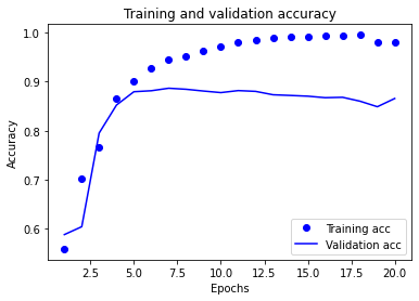
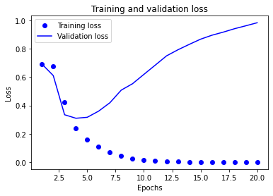
# model_2, history_2

acc2 = history_dict_2['accuracy']
val_acc2 = history_dict_2['val_accuracy']
loss2 = history_dict_2['loss']
val_loss2 = history_dict_2['val_loss']

epochs2 = range(1, len(acc2) + 1)

plt.plot(epochs2, loss2, 'bo', label='Training loss')

plt.plot(epochs2, val_loss2, 'b', label='Validation loss')
plt.title('Training and validation loss')
plt.xlabel('Epochs')
plt.ylabel('Loss')
plt.legend()

plt.show()
# Training and validation accuracy

# plt.clf()   # 그림을 초기화

plt.plot(epochs2, acc2, 'bo', label='Training acc')
plt.plot(epochs2, val_acc2, 'b', label='Validation acc')
plt.title('Training and validation accuracy')
plt.xlabel('Epochs')
plt.ylabel('Accuracy')
plt.legend()

plt.show()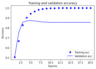
- Training and validation loss를 그려 보면, 몇 epoch까지의 트레이닝이 적절한지 최적점을 추정해 볼 수 있음
- validation loss의 그래프가 train loss와의 이격이 발생하게 되면 더 이상의 트레이닝은 무의미

:)