
📌 사용 환경
Python 3.10.2
conda 24.9.0
JupyterLab 4.2.5
1. 의사 결정 트리(Decision Tree)
요새 가장 많이 사용되는 의사결정트리(Decision Tree)다.
이 또한 분류와 회귀 둘 다 가능하며, 로지스틱 회귀와의 차이를 중점으로 설명한다.
먼저 필요한 라이브러리 import.
# 기본적인 부분
import numpy as np
import pandas as pd
import seaborn as sns
import matplotlib.pyplot as plt
import matplotlib as mpl
mpl.rc("font", family="Malgun Gothic")
plt.rcParams["axes.unicode_minus"]=False

# 데이터 전처리
from sklearn.model_selection import train_test_split
from sklearn.preprocessing import StandardScaler

# 학습 알고리즘
from sklearn.neighbors import KNeighborsRegressor
from sklearn.neighbors import KNeighborsClassifier

from sklearn.linear_model import LinearRegression
from sklearn.linear_model import LogisticRegression

from sklearn.metrics import classification_report
from scipy.special import expit, softmax

from sklearn.tree import DecisionTreeClassifier
from sklearn.tree import DecisionTreeRegressor
from sklearn.tree import plot_tree

from sklearn.model_selection import cross_validate
1.1. Decision Tree Classifier
비선형 관계 학습
스케일링이 필요 없음
해석이 쉽고 직관적인 모델
화이트 와인인지 레드 와인인지를 분류하는데
로지스틱 회귀를 먼저 보자.
https://raw.githubusercontent.com/rickiepark/hg-mldl/master/wine.csv
1.1.1. 와인 품종 분류 - 로지스틱 회귀
wine=pd.read_csv("./data/wine.csv")
wine.shape
(6497, 4)wine.head()| alcohol | sugar | pH | class | |
|---|---|---|---|---|
| 0 | 9.4 | 1.9 | 3.51 | 0.0 |
| 1 | 9.8 | 2.6 | 3.20 | 0.0 |
| 2 | 9.8 | 2.3 | 3.26 | 0.0 |
| 3 | 9.8 | 1.9 | 3.16 | 0.0 |
| 4 | 9.4 | 1.9 | 3.51 | 0.0 |
각각 알콜도수, 당도, 산도, 분류다.
0이 레드와인, 1이 화이트 와인이다.
wine.info()<class 'pandas.core.frame.DataFrame'>
RangeIndex: 6497 entries, 0 to 6496
Data columns (total 4 columns):
# Column Non-Null Count Dtype
--- ------ -------------- -----
0 alcohol 6497 non-null float64
1 sugar 6497 non-null float64
2 pH 6497 non-null float64
3 class 6497 non-null float64
dtypes: float64(4)
memory usage: 203.2 KB결측치 없고, 전부 실수형태다.
wine.describe().T| count | mean | std | min | 25% | 50% | 75% | max | |
|---|---|---|---|---|---|---|---|---|
| alcohol | 6497.0 | 10.491801 | 1.192712 | 8.00 | 9.50 | 10.30 | 11.30 | 14.90 |
| sugar | 6497.0 | 5.443235 | 4.757804 | 0.60 | 1.80 | 3.00 | 8.10 | 65.80 |
| pH | 6497.0 | 3.218501 | 0.160787 | 2.72 | 3.11 | 3.21 | 3.32 | 4.01 |
| class | 6497.0 | 0.753886 | 0.430779 | 0.00 | 1.00 | 1.00 | 1.00 | 1.00 |
wine["class"].value_counts()class
1.0 4898
0.0 1599
Name: count, dtype: int64화이트와인이 4898개로 많다.
이제 전체적으로 그래프를 보면,
sns.pairplot(data=wine, hue="class")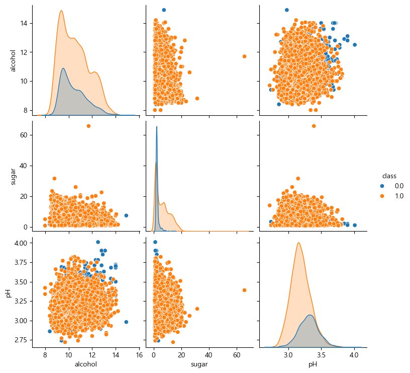
이런 그래프는 선형회귀로 하기 힘들다.
로지스틱 회귀는 선형회귀를 기반으로 해서 확률분포로 바꿔주는 건데,
선형회귀로 하기 힘드니까 예측이 잘 안나올 수 있다.
상관관계를 보면,
wine.corr().round(2)| alcohol | sugar | pH | class | |
|---|---|---|---|---|
| alcohol | 1.00 | -0.36 | 0.12 | 0.03 |
| sugar | -0.36 | 1.00 | -0.27 | 0.35 |
| pH | 0.12 | -0.27 | 1.00 | -0.33 |
| class | 0.03 | 0.35 | -0.33 | 1.00 |
상관관계도 그렇게 좋지 않다.
예측률이 낮을 것이다.
설명변수와 목표변수를 나눠주자.
X=wine.iloc[:,:3]
Y=wine.iloc[:,-1]
print(X.shape, type(X))
print(Y.shape, type(Y))
(6497, 3) <class 'pandas.core.frame.DataFrame'>
(6497,) <class 'pandas.core.series.Series'>이제 훈련과 학습데이터를 나누자.
X_train, X_test, Y_train, Y_test=train_test_split(X, Y, random_state=42)나눴으니 표준화
scaler=StandardScaler()
scaler.fit(X_train)

X_train_scaled=scaler.transform(X_train)
X_test_scaled=scaler.transform(X_test)
이제 로지스틱 회귀를 이용해서 학습시키자.
lr=LogisticRegression()
lr.fit(X_train_scaled, Y_train)
이제 학습을 시켰으니 정확도를 평가를 해보면,
print("학습: ", lr.score(X_train_scaled, Y_train))
print("일반화: ", lr.score(X_test_scaled, Y_test))
학습: 0.7859195402298851
일반화: 0.7655384615384615상관성이 낮은 편이었는데 괜찮게 나왔다.
Over나 Undder fitting도 아니다.
그렇다면 평가지표를 보자.
Y_test_pred=lr.predict(X_test_scaled)
print(classification_report(Y_test, Y_test_pred))
precision recall f1-score support
0.0 0.60 0.35 0.45 434
1.0 0.80 0.92 0.85 1191
accuracy 0.77 1625
macro avg 0.70 0.64 0.65 1625
weighted avg 0.74 0.77 0.74 16251의 경우는 아주 잘나왔는데, 0인 레드와인의 경우가 많이 떨어진다.
이런 경우 좋은 모델이 아니다.
데이터를 보니 상관성도 떨어지고, 모양도 선형이나 곡선이면 규제를 주면되듯이 해결방법이 있지만 그렇지 않고,
KNN으로 할 수도 있는데, KNN은 또 새로운 데이터에 의한 예측율이 떨어진다.
따라서 이런 문제 때문에 결정트리가 나온 것이다.
1.1.2. 와인 품종 분류 - Decision Tree Classifier
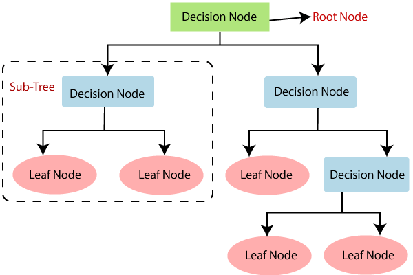
Decision Tree의 구조는 이와 같다.
-
Root Node는 모든 데이터의 정보를 가지고 있으며,
-
Decision Node에서 데이터를 분류할 질문을 한다.
이에 따라 True일 경우와 False일 경우로 나누는데,
이를 평가하는 기준으로 gini-index 와 Entropy를 사용한다.
이 중 gini-index에 대해서만 다룬다. -
다시 Sub Tree로 분류되어
그 안에서 또 다시 Decision Node에서 분류할 질문을 통해 T/F로 나눈다. -
이렇게 하여 의사결정을 하지 않는 마지막 노드가 Leaf Node이며 표현은 타원형으로 한다.
-
이때 각 Decision Node를 기준으로 depth라는 깊이로 표현하는데,
Root Node부터 Decision Node를 depth = 1,
첫번째 DecisionNode부터 두번째 Decision Node를 depth=2와 같이 진행하는데,
이 depth가 깊어질수록 조건이 세세하게 나뉘기 때문에
다항 회귀에서 훈련데이터들이 모든 점을 다 맞추게 되듯이 과대 적합이 된다. -
이제 데이터가 O가 50개, X가 50개가 있다고 가정해보자.
이를 평가기준으로 나눴는데, 왼쪽과 오른쪽 노드가 동일하게 O 25개, X 25개로 나뉜다면, 이는 완전 망한 것이다.
이는 KNN에서 n_neighbors를 홀수로 지정하는 이유와 같다.
똑같이 들어가면 안되며,
반대로 왼쪽노드에 O가 50개, X가 50개와 같이 들어가면 아주 잘한 순수 노드가 되는 것이다. -
이 순수 라는 말을 잘 알아야하는데,
앞서 depth가 깊어질수록 조건이 세세하게 나뉘면서 순수 노드에 가까워 지는데,
이렇게 순수 노드에 가까워 지는 것을 불순도(gini) 가 줄어든다고 한다.
즉 불순도란 O와 X가 섞인 것을 말하며,
이런 순수 노드에 가까워지며 불순도가 내려가는 것을 정보 이익(information Gain) 이라고 한다. -
그리고 이 불순도(gini) 는 데이터 분할의 기준이 된다.
- : 클래스의 개수
- : i번째 클래스에 속할 확률
지니 불순도가 낮을수록 데이터가 순수하다는 의미다.
이제 이를 코드를 보며 자세히 알아보자.
dt=DecisionTreeClassifier(random_state=42)
dt.fit(X_train_scaled, Y_train)
지금은 가지치기를 안했기에 학습율이 엄청 높을 것이다.
print("학습: ", dt.score(X_train_scaled, Y_train))
print("일반화: ", dt.score(X_test_scaled, Y_test))
학습: 0.9973316912972086
일반화: 0.8516923076923076로지스틱에 비해 완전 잘나왔다.
이를 시각화하면,
plt.figure(figsize=(10,7))
plot_tree(dt)
plt.show()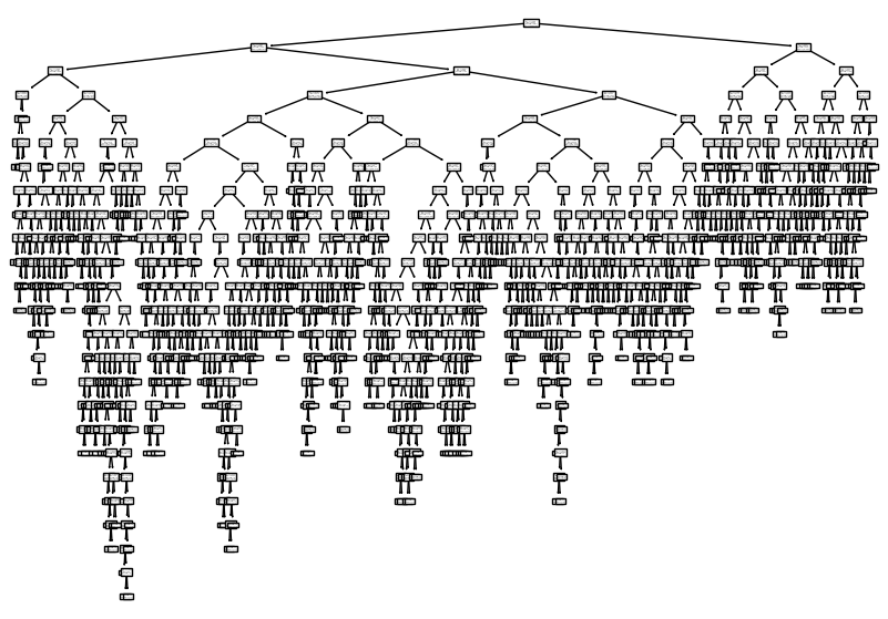
열이 3개인데 이만큼 나온다.
1.1.2.1. Gini 불순도
wine.corr().round(2)| alcohol | sugar | pH | class | |
|---|---|---|---|---|
| alcohol | 1.00 | -0.36 | 0.12 | 0.03 |
| sugar | -0.36 | 1.00 | -0.27 | 0.35 |
| pH | 0.12 | -0.27 | 1.00 | -0.33 |
| class | 0.03 | 0.35 | -0.33 | 1.00 |
plt.figure(figsize=(10,7))
plot_tree(dt, max_depth=1, filled=True, feature_names=["alchol", "sugar", "pH"])  # filed=True: 클래스마다 색깔 다르게
plt.show()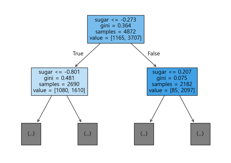
특성 중요도라는게 있는데,
dt.feature_importances_array([0.12871631, 0.86213285, 0.00915084])특성들의 중요도를 기준으로 나눠준다.
각각 alcohol, sugar, pH이며 sugar가 가장 크기 때문에 sugar가 테스트 조건으로 들어간 것이다.
그리고 -0.273은 훈련 데이터에서 sugar 값에 대해 여러 임계값을 시험한 후,
지니 불순도가가 가장 낮아지는 기준값으로 계산된 값이다.
즉, 결정 트리는 훈련 데이터의 sugar 값들을 이용해
sugar <= -0.273이 불순도가 가장 낮은 분할 기준으로 선택했다고 볼 수 있다.
따라서 이제 이를 기준으로 test가 들어오면, 이에 맞춰서 왼쪽 노드나 오른쪽 노드로 나눠주는 것이다.
1.1.2.2. 가지치기
과대적합 방지
앞서 DecisionTreeClassifier 생성자를 만들때, 그냥 사용했는데,
과대 적합을 방지하기위해 가지 치기를 결정할 수 있다.
dt=DecisionTreeClassifier(max_depth=3, random_state=42)
dt.fit(X_train_scaled, Y_train)
이렇게 max_depth를 지정 해줘서 depth=3 까지만 가지친다.
그래서 이렇게 한 후 평가해보면,
print("학습: ", dt.score(X_train_scaled, Y_train))
print("일반화: ", dt.score(X_test_scaled, Y_test))
학습: 0.8499589490968801
일반화: 0.8363076923076923그리고 이를 시각화해보면,
plt.figure(figsize=(20,15))
plot_tree(dt, filled=True, feature_names=["alcohole", "sugar", "pH"])
plt.show()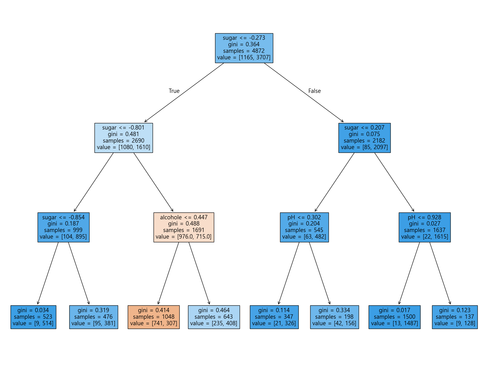
이렇게 나온다.
따라서 만약, 새로운 테스트 데이터가 들어온 후,
F->T->F로 간다면, value=[42,156] 이기 때문에 더 큰 156인 white 와인이 되는 것이다.
Y_test_pred=dt.predict(X_test_scaled)
print(classification_report(Y_test, Y_test_pred))
precision recall f1-score support
0.0 0.73 0.61 0.67 434
1.0 0.87 0.92 0.89 1191
accuracy 0.84 1625
macro avg 0.80 0.77 0.78 1625
weighted avg 0.83 0.84 0.83 16251.1.3. 스케일 조정을 하지 않는 특성 사용
wine=pd.read_csv("./data/wine.csv")
wine.shape
(6497, 4)X=wine.iloc[:, :3]
Y=wine.iloc[:, -1]
X.shape, Y.shape((6497, 3), (6497,))X_train, X_test, Y_train, Y_test=train_test_split(X,Y,random_state=42)이번에는 이렇게 표준화하지 않고 바로 사용한다.
max_depth=5로 둔다.
dt=DecisionTreeClassifier(max_depth=5, random_state=42)
dt.fit(X_train, Y_train)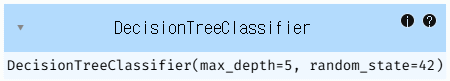
평가해주면,
print("학습: ", dt.score(X_train, Y_train))
print("일반화: ", dt.score(X_test, Y_test))학습: 0.8725369458128078
일반화: 0.8584615384615385Y_test_pred=dt.predict(X_test)
print(classification_report(Y_test, Y_test_pred)) precision recall f1-score support
0.0 0.73 0.74 0.74 434
1.0 0.90 0.90 0.90 1191
accuracy 0.86 1625
macro avg 0.82 0.82 0.82 1625
weighted avg 0.86 0.86 0.86 1625특성중요도를 보면,
dt.feature_importances_array([0.13860406, 0.72615713, 0.1352388 ])plt.figure(figsize=(20, 15))
plot_tree(dt, filled=True, feature_names=["alcohol","sugar","pH"])
plt.show()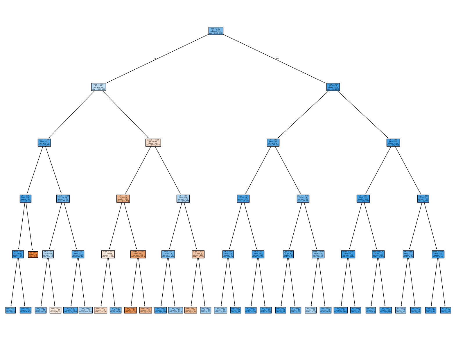
1.2. Decision Tree Regression
1.2.1. Kaggle 서울 아파트 가격 예측
https://www.kaggle.com/datasets/jcy1996/seoul-real-estate-datasets
서울 아파트의 평균 가격을 예측해보자.
1.2.1.1. 데이터 전처리
apart=pd.read_csv("./data/seoulapartment.csv")
apart.shape(4544, 11)apart.head()| index | name | gugun | dong | buildDate | min_sales | max_sales | avg_sales | area | floor | pricePerArea | |
|---|---|---|---|---|---|---|---|---|---|---|---|
| 0 | 0 | 수락산벨리체 | 노원구 | 상계동 | 200006.0 | 97000.0 | 107000.0 | 101000.0 | 139 | 42 | 697.841727 |
| 1 | 1 | 수락파크빌 | 노원구 | 상계동 | 200105.0 | 83000.0 | 92000.0 | 89000.0 | 105 | 32 | 790.476191 |
| 2 | 2 | 비콘드림힐2차 | 노원구 | 상계동 | 200502.0 | 62000.0 | 74000.0 | 71500.0 | 86 | 26 | 720.930233 |
| 3 | 3 | 수락현대 | 노원구 | 상계동 | 199509.0 | 65000.0 | 66000.0 | 65500.0 | 102 | 31 | 637.254902 |
| 4 | 4 | 대망드림힐 | 노원구 | 상계동 | 200306.0 | 63000.0 | 78000.0 | 70000.0 | 91 | 28 | 692.307692 |
apart.info()<class 'pandas.core.frame.DataFrame'>
RangeIndex: 4544 entries, 0 to 4543
Data columns (total 11 columns):
# Column Non-Null Count Dtype
--- ------ -------------- -----
0 index 4544 non-null int64
1 name 4544 non-null object
2 gugun 4544 non-null object
3 dong 4544 non-null object
4 buildDate 4462 non-null float64
5 min_sales 4333 non-null float64
6 max_sales 4333 non-null float64
7 avg_sales 4333 non-null float64
8 area 4544 non-null int64
9 floor 4544 non-null int64
10 pricePerArea 4333 non-null float64
dtypes: float64(5), int64(3), object(3)
memory usage: 390.6+ KB여기서 평균 가격인 avg_sales를 예측할 것이다.
그런데 우선 결측치가 있으니 지워주자.
apart_copy=apart.copy()apart_copy.dropna(inplace=True)apart_copy.info()<class 'pandas.core.frame.DataFrame'>
Index: 4333 entries, 0 to 4543
Data columns (total 11 columns):
# Column Non-Null Count Dtype
--- ------ -------------- -----
0 index 4333 non-null int64
1 name 4333 non-null object
2 gugun 4333 non-null object
3 dong 4333 non-null object
4 buildDate 4333 non-null float64
5 min_sales 4333 non-null float64
6 max_sales 4333 non-null float64
7 avg_sales 4333 non-null float64
8 area 4333 non-null int64
9 floor 4333 non-null int64
10 pricePerArea 4333 non-null float64
dtypes: float64(5), int64(3), object(3)
memory usage: 406.2+ KBapart_copy.describe().round(2).T| count | mean | std | min | 25% | 50% | 75% | max | |
|---|---|---|---|---|---|---|---|---|
| index | 4333.0 | 78.56 | 54.60 | 0.00 | 34.00 | 71.00 | 114.00 | 270.00 |
| buildDate | 4333.0 | 199993.78 | 1128.76 | 196506.00 | 199406.00 | 200209.00 | 200701.00 | 202109.00 |
| min_sales | 4333.0 | 86738.20 | 68812.42 | 1200.00 | 39000.00 | 71000.00 | 114000.00 | 591000.00 |
| max_sales | 4333.0 | 126333.76 | 113623.71 | 3700.00 | 56000.00 | 94000.00 | 157000.00 | 974000.00 |
| avg_sales | 4333.0 | 103383.22 | 81972.17 | 3300.00 | 48000.00 | 82000.00 | 135000.00 | 636000.00 |
| area | 4333.0 | 85.88 | 31.52 | 13.00 | 71.00 | 82.00 | 101.00 | 281.00 |
| floor | 4333.0 | 25.99 | 9.54 | 4.00 | 21.00 | 25.00 | 31.00 | 85.00 |
| pricePerArea | 4333.0 | 971.52 | 597.95 | 36.36 | 556.82 | 853.66 | 1273.81 | 3204.55 |
apart_copy.describe(include="object")| name | gugun | dong | |
|---|---|---|---|
| count | 4333 | 4333 | 4333 |
| unique | 2469 | 30 | 300 |
| top | 현대 | 강남구 | 삼성동 |
| freq | 45 | 637 | 153 |
지금은 지역은 신경쓰지 않지만,
만약 gugun으로 하면 원핫 인코딩으로 1 0 0 0 0 0 ... 처럼 30개가 되며,
dong으로 하면 300개를 해야한다.
gugun으로하자.
상관분석을 진행하자.
apart_copy_num=apart_copy.select_dtypes(include="number")
apart_copy_num.corr().round(2).abs()| index | buildDate | min_sales | max_sales | avg_sales | area | floor | pricePerArea | |
|---|---|---|---|---|---|---|---|---|
| index | 1.00 | 0.03 | 0.16 | 0.15 | 0.17 | 0.08 | 0.08 | 0.14 |
| buildDate | 0.03 | 1.00 | 0.08 | 0.12 | 0.09 | 0.16 | 0.16 | 0.08 |
| min_sales | 0.16 | 0.08 | 1.00 | 0.87 | 0.96 | 0.62 | 0.62 | 0.83 |
| max_sales | 0.15 | 0.12 | 0.87 | 1.00 | 0.95 | 0.48 | 0.48 | 0.78 |
| avg_sales | 0.17 | 0.09 | 0.96 | 0.95 | 1.00 | 0.54 | 0.54 | 0.85 |
| area | 0.08 | 0.16 | 0.62 | 0.48 | 0.54 | 1.00 | 1.00 | 0.18 |
| floor | 0.08 | 0.16 | 0.62 | 0.48 | 0.54 | 1.00 | 1.00 | 0.18 |
| pricePerArea | 0.14 | 0.08 | 0.83 | 0.78 | 0.85 | 0.18 | 0.18 | 1.00 |
avg_sales 중 자신을 제외하고, 의미없는 min, max도 제외하고, 날짜도 제외
남는 area, fllot, pricePerArea를 가져다 쓰면 된다.
apart_copy.columnsIndex(['index', 'name', 'gugun', 'dong', 'buildDate', 'min_sales', 'max_sales',
'avg_sales', 'area', 'floor', 'pricePerArea'],
dtype='object')X=apart_copy[["area", "floor", "pricePerArea"]]
Y=apart_copy["avg_sales"]
X.shape, Y.shape((4333, 3), (4333,))이제 시각화를 할 것인데, X와 Y를 다 그릴수는 없다.
2차원까지만 그릴 수 있기 때문에.
fig, axes=plt.subplots(nrows=1, ncols=3, figsize=(20,5)) # 1행 3열
sns.scatterplot(data=apart_copy, x="area", y="avg_sales", ax=axes[0])
sns.scatterplot(data=apart_copy, x="floor", y="avg_sales", ax=axes[1])
sns.scatterplot(data=apart_copy, x="pricePerArea", y="avg_sales", ax=axes[2])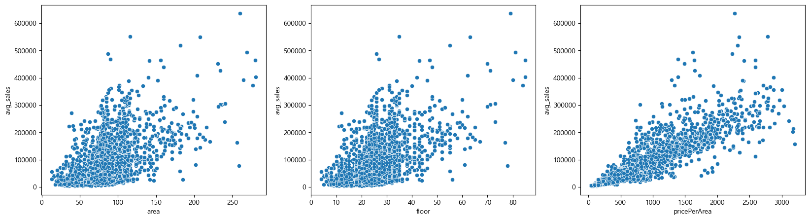
이렇게 직선과 얼추 비슷하게 나온다.
이제 선형회귀와 KNR를 해보고 결정트리회귀 모델까지 해보자.
먼저 각각 진행하기 전에 학습데이터와 테스트 데이터까지 나눠놓고 각각 가져다 사용하자.
X_train, X_test, Y_train, Y_test=train_test_split(X,Y,random_state=42)scaler=StandardScaler()
scaler.fit(X_train)
X_train_scaled=scaler.transform(X_train)
X_test_scaled=scaler.transform(X_test)1.2.1.2. Linear Regression
lr=LinearRegression()
lr.fit(X_train_scaled, Y_train)
print("학습: ", lr.score(X_train_scaled, Y_train))
print("일반화: ", lr.score(X_test_scaled, Y_test))학습: 0.8791185845564701
일반화: 0.8787512977138664앞서 시각화로 봤듯이 직선과 얼추 비슷하게 나왔기 때문에
이 선형회귀모델에서의 값이 괜찮게 잘 나온다.
1.2.1.3. KNR
kn=KNeighborsRegressor()
kn.fit(X_train_scaled, Y_train)
print("학습: ", kn.score(X_train_scaled, Y_train))
print("일반화: ", kn.score(X_test_scaled, Y_test))학습: 0.9572401881915524
일반화: 0.9447525773202533비슷한 애들을 보기때문에 KNR이 점수가 잘 나온다.
1.2.1.4. Decision Tree Regression
얘는 계산이 아니라 트리로 좌로 갈지 우로갈지를 정하기 때문에 scale을 빼서 진행한다.
dt=DecisionTreeRegressor(max_depth=5, random_state=42)
dt.fit(X_train, Y_train)
print("학습: ", dt.score(X_train, Y_train))
print("일반화: ", dt.score(X_test, Y_test))학습: 0.9236594039095398
일반화: 0.912419150210737490퍼센트 이상으로 잘 나왔다.
트리를 한번 보자.
먼저 특성 중요도를 보자.
dt.feature_importances_array([0.17812679, 0.01909403, 0.80277919])마지막인 pricePeraArea가 들어갈 것이다.
그리고 depth를 5까지 줘서 학습한 모델에서 시각화는 depth=1까지만 보면,
plt.figure(figsize=(15,5))
plot_tree(dt, max_depth=1, filled=True, feature_names=["area", "floor", "pricePerArea"])
plt.show()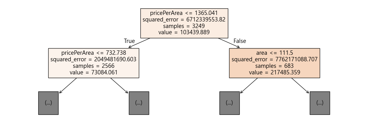
그런데 이렇게 max_depth와 같은 하이퍼 파라미터값을 잘 조절해야 과대적합이 일어나지 않는다.
따라서 이번에는 모델 최적화에 대해 알아보자.
2. 모델 최적화
교차검증, 하이퍼파라미터(HyperParameter)
2.1. 교차검증
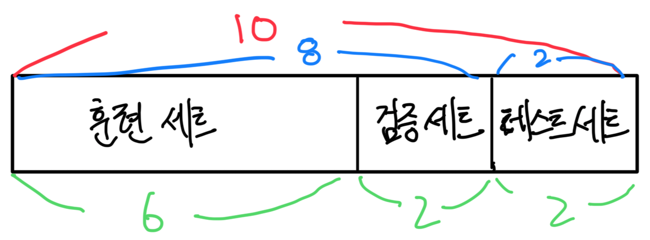
지금까지 전체 데이터에서 훈련 데이터와 테스트 데이터를 7:3이나 8:2로 나눴었는데
이번에는 검증(validation) 데이터라는 것을 한세트를 더 만든다.
테스트 데이터는 그대로 가져가고 훈련 데이터에서 검증(validation) 데이터를 또 8:2로 쪼개서 나눠서 주는 것이다.
즉 전체로 보면, 6:2:2 가 될 것이다.
그런데 이제 나누고 훈련을 할때 방법이 좀 다르다.
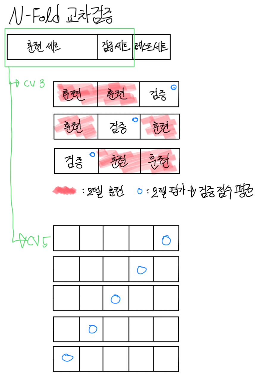
이렇게 지금까지는 훈련을 쭉 하고 테스트로 확인해봤었는데,
이번에는 이렇게 훈련과 테스트를 나눈 다음
또다시 훈련을 cv=3, 5개 이런식으로 나눠서
훈련 세트로 모델 훈련을 하고,
검증 세트로 모델 평가를 한 다음에 이 검증 점수의 평균이 나오는 것이다.
단 이렇게 훈련세트를 또 검증 세트로 나누는 것이기 때문에, 데이터가 많지 않으면 겹치는 부분이 생길 수 있다.
앞서 와인데이터를 로지스틱이랑 결정트리로 해봤으니 이번에는 KNN으로 테스트해보자.
wine=pd.read_csv("./data/wine.csv")
wine.shape(6497, 4)X=wine.iloc[:,:3]
Y=wine.iloc[:,-1]
X.shape, Y.shape((6497, 3), (6497,))X_train, X_test, Y_train, Y_test=train_test_split(X,Y,test_size=0.2,random_state=42) # 검증데이터를 또 나눠줘야하니까 8:2로 조절scaler=StandardScaler()
scaler.fit(X_train)
X_train_scaled=scaler.transform(X_train)
X_test_scaled=scaler.transform(X_test)knn=KNeighborsClassifier(n_neighbors=5)
knn.fit(X_train_scaled, Y_train)
이제 모델 학습까지 끝나서 교차 검증을 진행한다.
그러면 이제 먼저 8:2로 나눈 데이터의 8부분을 다시 훈련과 검증 데이터로 또 나누는 것이다.
cross_validate라는 함수를 사용해야하며 import가 필요하다.
from sklearn.model_selection import cross_validateval_data=cross_validate(knn, X_train_scaled, Y_train, cv=5)cross_validate라는 교차검증 함수를 사용하여 평가하며, 5-fold 교차 검증이라고 한다.
이때 파라미터로 knn모델과 표준화를 진행한 모델 훈련 데이터, 그리고 마지막으로 cv값이 들어가는데,
여기서 cv란 앞서 설명한 것과 같이 5개로 나누는 것이다.
그리고 이렇게 하면 내부적으로 알아서 검증 데이터를 20%로 할당해서 나눠준다.
만약 cv=3이라면 33.3%정도로 나눈다.
val_data{'fit_time': array([0.00698113, 0.00600314, 0.00598168, 0.00598478, 0.00498605]),
'score_time': array([0.0709064 , 0.06238699, 0.0518899 , 0.0510149 , 0.05487323]),
'test_score': array([0.84903846, 0.85384615, 0.87487969, 0.86236766, 0.85370549])}이렇게 하여 실제 값은 test_score이다.
즉, test_score는 데이터에 대해 모델의 성능을 평가한 정확도이며,
fit_time은 모델 학습에 소요된 시간,
score_time은 테스트 데이터에 대한 점수를 계산하는데 걸리는 시간이다.
print("학습: ", knn.score(X_train_scaled, Y_train))
print("검증: ", val_data["test_score"].mean()) # key-value로 접근하여 값들의 평균, 즉 교차 검증의 평균
print("일반화: ", knn.score(X_test_scaled, Y_test))학습: 0.90186646142005
검증: 0.8587674909306285
일반화: 0.8338461538461538이번에는 7-fold 교차 검증을 사용해 모델을 평가해보자.
그리고 교차검증을 진행하기전에 cross_validate 함수의 내부에 알아할 부분이 있다.
만약 cv가 5고, 훈련데이터가 10000개라면, 8000개의 훈련, 2000개의 검증 데이터가 5번 반복(n개 * 5번)되는 것인데,
그러면 총 50000개를 돌리는 것이다.
그런데 만약 이게 10만개, 100만개가 된다면 어떨까?
이럴 때를 위해서 CPU의 코어를 사용하여 계산을 돕게할 수 있다.
이걸 지정해주는 것이 n_jobs다.
# n_jobs=-1: CPU 코어 다 사용
# return_train_score=True: 훈련 점수도 return
scores=cross_validate(knn, X_train_scaled, Y_train, cv=7, n_jobs=-1, return_train_score=True)
print("각 fold의 훈련 정확도: ", scores["train_score"])
print("훈련 평균: ", scores["train_score"].mean())
print()
print("각 fold의 검증 정확도: ", scores["test_score"])
print("검증 평균: ", scores["test_score"].mean())각 fold의 훈련 정확도: [0.90278401 0.89649753 0.90435564 0.9010101 0.9030303 0.90213244
0.90258137]
훈련 평균: 0.9017701984024392
각 fold의 검증 정확도: [0.85195155 0.8640646 0.85733513 0.8787062 0.87331536 0.8638814
0.86522911]
검증 평균: 0.86492619343885252.2. 하이퍼파라미터(HyperParameter)
모델 파라미터: 머신러닝 모델이 학습할 수 있도록 만든 파라미터
하이퍼 파라미터: 사용자가 지정하는 파라미터(i.g., n_neighbors)
릿지, 라소에서 0으로 너무 잘 맞추니까 cost함수를 올리는 방법을 이용했고,
그래서 최적의 파라미터를 찾기 위해 for문을 돌렸고,
KNN에서는 n_neighbors를 조절했었다.
그래서 그 중 골라서 사용했어야 했는데,
교차 검증과 하이퍼파라미터 탐색까지 한번에 자동으로 해주는 클래스인 GridSearchCV 가 있다.
2.2.1. GridSearch
하이퍼파라미터 범위 설정
하이퍼파라미터 탐색 실행 + 교차 검증
최적의 조합을 찾아서 반환
2.2.1.1. KNeighbors
먼저 KNN에서의 경우를 보자.
와인 데이터를 그대로 이용한다.
wine=pd.read_csv("./data/wine.csv")
X=wine.iloc[:,:3]
Y=wine.iloc[:,-1]
X.shape, Y.shape((6497, 3), (6497,))이제 학습과 테스트 데이터 셋을 나누고,
X_train, X_test, Y_train, Y_test=train_test_split(X,Y,test_size=0.2,random_state=42) # 8:2표준화를 진행한다.
scaler=StandardScaler()
scaler.fit(X_train)
X_train_scaled=scaler.transform(X_train)
X_test_scaled=scaler.transform(X_test)여기까지는 똑같지만 이제 모델을 학습할때 과정이 달라진다.
먼저 탐색할 파라미터를 설정한다.
params={"n_neighbors":[3,5,7,9,11]} # params={"n_neighbors":np.arange(3,12,2)}그리고 이제 GridSearch를 초기화 해줘야한다.
이 GridSearch를 사용하기 위해서는 import가 필요하다.
from sklearn.model_selection import GridSearchCVgs=GridSearchCV(KNeighborsClassifier(), params, cv=5, n_jobs=-1)이제 이 이 gs의 fit을 사용하여 최적의 파라미터를 찾는다.
gs.fit(X_train_scaled, Y_train)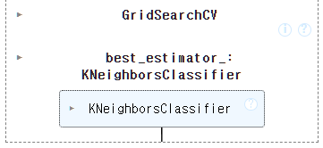
이제 최적의 매개 변수와, 최적의 교차 검증 점수를 확인해보자.
gs.best_params_{'n_neighbors': 5}gs.best_score_np.float64(0.8587674909306285)이 모델에서 교차검증 점수가 가장 높은게 85점인 것이다.
그리고 이제 나온 최적의 모델로 테스트 데이터를 평가해야한다.
knn_best=gs.best_estimator_
knn_best.score(X_test_scaled, Y_test)0.8338461538461538훈련 85점, 테스트 83점이니까 잘 나온 것이다.
이제 예측값을 넣어 평가지표를 보자.
Y_test_pred=gs.predict(X_test_scaled)
print(classification_report(Y_test, Y_test_pred)) precision recall f1-score support
0.0 0.70 0.65 0.67 341
1.0 0.88 0.90 0.89 959
accuracy 0.83 1300
macro avg 0.79 0.77 0.78 1300
weighted avg 0.83 0.83 0.83 13002.2.1.2. DecisionTree
이번에는 의사결정트리에서의 경우를 보자.
그런데 이 의사결정트리는 지정해줄 파라미터가 꽤 있다.
DecisionTreeClassifier().get_params(){'ccp_alpha': 0.0,
'class_weight': None,
'criterion': 'gini',
'max_depth': None,
'max_features': None,
'max_leaf_nodes': None,
'min_impurity_decrease': 0.0,
'min_samples_leaf': 1,
'min_samples_split': 2,
'min_weight_fraction_leaf': 0.0,
'monotonic_cst': None,
'random_state': None,
'splitter': 'best'}
이들 중 3가지 정도를 많이 쓰는데,
- max_depth: 가지치기, 트리의 최대 길이
- min_impurity_decrease: gini 불순도 값이 끝나는 기준(default인 0이면 끝까지 가서 과대적합일어나니까 조정필요)
- min_samples_split: 나눌때 그냥 나누는 게 아니라, 셈플수가 있어야 나눌 수 있다. 이를 지정해준다. 노드분할에 필요한 최소 셈플수
wine=pd.read_csv("./data/wine.csv")
X=wine.iloc[:,:3]
Y=wine.iloc[:,-1]
X.shape, Y.shape((6497, 3), (6497,))X_train, X_test, Y_train, Y_test=train_test_split(X,Y,test_size=0.2,random_state=42)그리고 이는 트리이기때문에 스케일링을 안해도 된다.
params를 만들자.
params={
"max_depth": np.arange(5, 20),
"min_impurity_decrease": np.arange(0.0001, 0.0006, 0.0001),
"min_samples_split": np.arange(2, 100, 2)
}이제 만든 params를 넣어서 fit을 사용하여 최적의 파라미터를 찾아주자.
gs=GridSearchCV(DecisionTreeClassifier(random_state=42), params, n_jobs=-1, cv=5)
gs.fit(X_train, Y_train)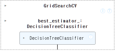
최적의 매개 변수는,
gs.best_params_{'max_depth': np.int64(14),
'min_impurity_decrease': np.float64(0.0004),
'min_samples_split': np.int64(8)}교차 검증의 점수는
gs.best_score_np.float64(0.8689635004071963)그리고 이제 best를 뽑아와서 테스트 데이터로 최적의 모델을 평가하면,
gs_best=gs.best_estimator_
gs_best.score(X_test, Y_test)0.8615384615384616Y_test_pred=gs.predict(X_test)
print(classification_report(Y_test, Y_test_pred)) precision recall f1-score support
0.0 0.74 0.73 0.73 341
1.0 0.90 0.91 0.91 959
accuracy 0.86 1300
macro avg 0.82 0.82 0.82 1300
weighted avg 0.86 0.86 0.86 1300여태까지 중에 가장 최적을 보인다.
2.2.2. RandomSearch
랜덤 서치라는 것이 있다.
GridSearch는 지정해준 값들의 조합을 전부 다 돌리면서 알아서 최적을 뽑아낸다.
RandomSearch는 지정해준 하이퍼파라미터 구간에서 무작위로 값을 선택하여 조합을 만든다.
하나하나 돌려서 최적의 파라미터를 뽑는게 아니라, 값을 주고서 랜덤하게 뽑아내는 것이다.
예를들어 최적의 파라미터가 100이라고 하면, 1~500으로 지정하면, 다 돌면서 가장 좋은 트레이닝 학습율을 100으로 찾아서 리턴해주는데,
RandomSearch는 수의 범위를 1~500으로 지정하고 랜덤하게 찾게하는 것이다.
랜덤하게 100, 200, 등을 돌려보다가 100이 가장 좋다고 반환하는 것이다.
즉 데이터가 많지 않으면 GridSearch를 사용하는 것이 좋고 정확도가 높으며,
데이터가 많고 하이퍼파라미터의 구간이 많으면 랜덤이 더 빠르고 괜찮게 찾는다.
실무에서는 데이터가 워낙 많으니 RandomSearch를 많이 사용한다.
라이브러리 import가 필요하다.
from sklearn.model_selection import RandomizedSearchCV
from scipy.stats import uniform, randint혹은 그냥 np.random.uniform(), np.random.randint()를 사용해도 된다.
2.2.2.1. DecisionTree
parmas를 지정해주자.
params={
"max_depth":randint(5,20),
"min_impurity_decrease":uniform(0.0001, 0.0006), # 0.0001과 0.0006 사이의 랜덤 실수 생성
"min_samples_split":randint(2,100)
}rs=RandomizedSearchCV(DecisionTreeClassifier(random_state=42), params, n_jobs=-1, n_iter=100)
rs.fit(X_train, Y_train)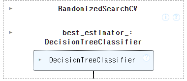
여기서 n_iter라는 게 있는데, n_iter가 100이면 100개의 조합을 랜덤하게 뽑으라는 것이다.
최적의 파라미터를 찾자.
rs.best_params_{'max_depth': 13,
'min_impurity_decrease': np.float64(0.0005191415748033069),
'min_samples_split': 13}
교차 검증 점수는,
rs.best_score_np.float64(0.8683863922410602)이제 best를 뽑아와서 테스트 데이터로 최적 모델 평가
rs_best=rs.best_estimator_
rs_best.score(X_test, Y_test)0.8615384615384616Y_test_pred=rs.predict(X_test)
print(classification_report(Y_test, Y_test_pred)) precision recall f1-score support
0.0 0.72 0.77 0.74 341
1.0 0.92 0.89 0.91 959
accuracy 0.86 1300
macro avg 0.82 0.83 0.82 1300
weighted avg 0.86 0.86 0.86 1300속도도 빠르고 점수도 잘 나왔다.
2.2.2.2. KNN
이번에는 KNN의 경우다.
X_train, X_test, Y_train, Y_test=train_test_split(X,Y,test_size=0.2,random_state=42) # 8:2scaler=StandardScaler()
scaler.fit(X_train)
X_train_scaled=scaler.transform(X_train)
X_test_scaled=scaler.transform(X_test)파라미터를 확인하자.
KNeighborsClassifier().get_params(){'algorithm': 'auto',
'leaf_size': 30,
'metric': 'minkowski',
'metric_params': None,
'n_jobs': None,
'n_neighbors': 5,
'p': 2,
'weights': 'uniform'}
이제 파라미터를 지정해주자.
params={
'n_neighbors': np.arange(1, 10, 2),
'weights': ['uniform', 'distance'],
'p': [1, 2]
}원래 KNN을 사용할때는 기본적으로 가중치 부여 방식을 uniform, 거리계산 p값을 유클리디안(2), n_neighbors도 5를 사용했었는데,
이번에는 이각 방식을 RandomSearch에서 선택해서 최적을 뽑아내도록 해보자.
rs=RandomizedSearchCV(KNeighborsClassifier(), params, n_iter=10, cv=5, n_jobs=-1)
rs.fit(X_train_scaled, Y_train)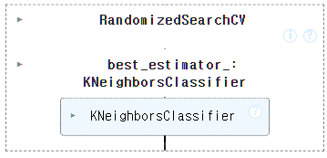
가장 좋은 성능을 낸 모델 반환해보면,
rs.best_estimator_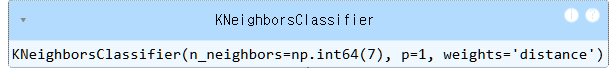
rs.best_params_{'weights': 'distance', 'p': 1, 'n_neighbors': np.int64(7)}이를 보니 n_neighbors는 7, 그리고 맨하탄, distance방식이 최적이다.
rs.best_score_np.float64(0.8807042644554676)이제 best를 뽑아서 테스트 데이터로 최적 모델 평가
knn_best=rs.best_estimator_
knn_best.score(X_test_scaled, Y_test)0.8653846153846154Y_test_pred=rs.predict(X_test_scaled)
print(classification_report(Y_test, Y_test_pred)) precision recall f1-score support
0.0 0.76 0.70 0.73 341
1.0 0.90 0.92 0.91 959
accuracy 0.87 1300
macro avg 0.83 0.81 0.82 1300
weighted avg 0.86 0.87 0.86 13003. Ensemble
이제 가장 중요한 앙상블(Ensemble)이다.
앙상블이란, 여러개의 개별 모델들을 결합해서 하나의 강력한 예측 모델을 만드는 것으로,
각 개별 모델들은 같은 종류가 될 수도 있고, 다른 종류가 될 수도 있다.
(의사 결정 트리, 로지스틱 회귀, K최근접 등)
이런 앙상블은 주로 분류 문제에서 많이 사용되지만 회귀에서도 사용 가능하다.
각 개별 모델들을 결합할때는 방법이 3가지가 있는데,
- 보팅(Voting): 서로 다른 알고리즘을 가진 여러 개의 모델을 사용하여 예측을 결합한다.
- 이 보팅에는 다수결을 뽑는 Hard 보팅과 예측 확률의 평균을 구하는 Soft보팅이 있다.
총 4개의 모델이 있다고 가정하자.- Hard 보팅: 모델 4개가 각각 1과 2에 대해서, 1, 2, 1, 1로 예측하면 다수결로 1로 예측한다.
- Soft 보팅: 모델 4개가 각각 1과 2에 대해서 예측 확률로, [0.7, 0.3], [0.2, 0.8], [0.8, 0.2], [0.9, 0.1]을 냈다면,
1로 예측한 값들의 평균 -> 0.7+0.2+0.8+0.9/4 = 0.65
2로 예측한 값들의 평균 -> 0.3+0.8+0.2+0.1/4 = 0.35
이 되어, 0.65>0.35 -> 0.65 -> 즉 1로 예측한다.
- 이 보팅에는 다수결을 뽑는 Hard 보팅과 예측 확률의 평균을 구하는 Soft보팅이 있다.
- 배깅(Bagging): 같은 알고리즘을 가진 여러 개의 모델을 사용하지만, 훈련 데이터셋을 무작위로 부분 샘플링하며,
여러 개의 부분 모델을 학습하여 평균 또는 다수결을 통해 예측한다.
이를 랜덤 포레스트 라고 하며 가장 꽃이 되는 방법이다.
먼저 필요한 라이브러리를 import해주고,
# 기본적인 부분
import numpy as np
import pandas as pd
import seaborn as sns
import matplotlib.pyplot as plt
import matplotlib as mpl
mpl.rc("font", family="Malgun Gothic")
plt.rcParams["axes.unicode_minus"]=False
# 데이터 전처리
from sklearn.model_selection import train_test_split
from sklearn.preprocessing import StandardScaler
# 학습 알고리즘
from sklearn.neighbors import KNeighborsClassifier, KNeighborsRegressor
from sklearn.linear_model import LinearRegression, LogisticRegression
from sklearn.tree import DecisionTreeClassifier, DecisionTreeRegressor
from sklearn.tree import plot_tree
from sklearn.model_selection import cross_validate, GridSearchCV, RandomizedSearchCV
from sklearn.ensemble import VotingClassifier
from sklearn.metrics import classification_report
from scipy.special import expit, softmax
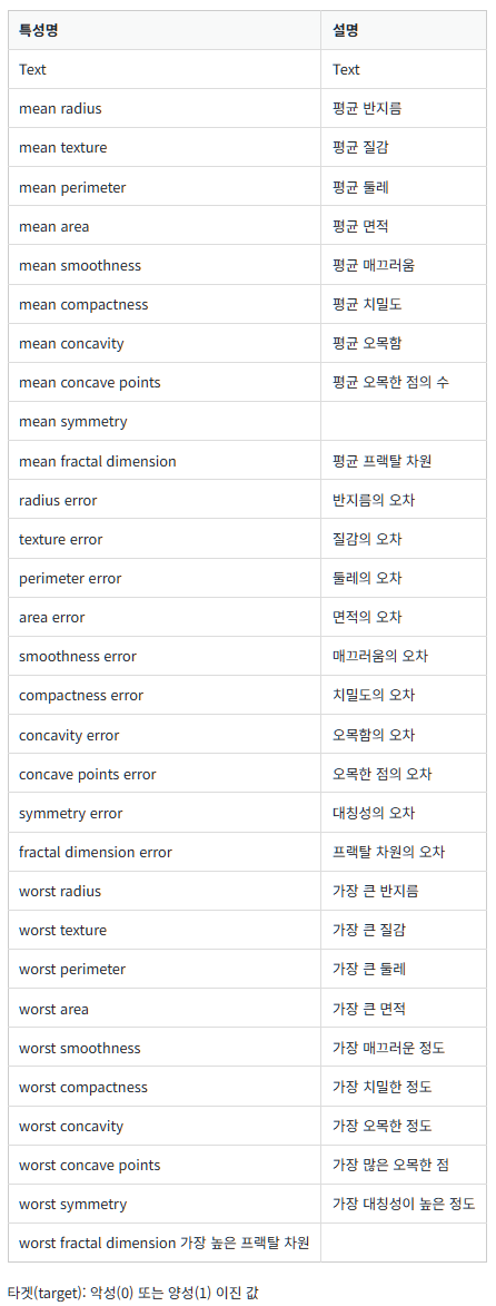
from scipy.stats import uniform, randint이번에는 사이킷런에서 제공하는 유방암 분류 예측을 해보자.
from sklearn.datasets import load_breast_cancer이 데이터셋에는 아주 많은 변수들이 있는데, 해석은 아래 사진을 참고하면 된다.
3.1. Voting
3.1.1. 데이터 전처리
cancer=load_breast_cancer()
type(cancer)sklearn.utils._bunch.Bunchdata, target=cancer.data, cancer.target
data.shape, target.shape((569, 30), (569,))이는 그런데 앞서 붓꽃 데이터때와 마찬가지로 사이킷런에서 제공한 데이터셋이 타입을 보면 bunch(numpy)로 되어있기 때문에 데이터프레임으로 변환해주자.
cancer_df=pd.DataFrame(data=cancer.data, columns=cancer.feature_names)
cancer_df["label"]=cancer.target
cancer_df.head()| mean radius | mean texture | mean perimeter | mean area | mean smoothness | mean compactness | mean concavity | mean concave points | mean symmetry | mean fractal dimension | ... | worst texture | worst perimeter | worst area | worst smoothness | worst compactness | worst concavity | worst concave points | worst symmetry | worst fractal dimension | label | |
|---|---|---|---|---|---|---|---|---|---|---|---|---|---|---|---|---|---|---|---|---|---|
| 0 | 17.99 | 10.38 | 122.80 | 1001.0 | 0.11840 | 0.27760 | 0.3001 | 0.14710 | 0.2419 | 0.07871 | ... | 17.33 | 184.60 | 2019.0 | 0.1622 | 0.6656 | 0.7119 | 0.2654 | 0.4601 | 0.11890 | 0 |
| 1 | 20.57 | 17.77 | 132.90 | 1326.0 | 0.08474 | 0.07864 | 0.0869 | 0.07017 | 0.1812 | 0.05667 | ... | 23.41 | 158.80 | 1956.0 | 0.1238 | 0.1866 | 0.2416 | 0.1860 | 0.2750 | 0.08902 | 0 |
| 2 | 19.69 | 21.25 | 130.00 | 1203.0 | 0.10960 | 0.15990 | 0.1974 | 0.12790 | 0.2069 | 0.05999 | ... | 25.53 | 152.50 | 1709.0 | 0.1444 | 0.4245 | 0.4504 | 0.2430 | 0.3613 | 0.08758 | 0 |
| 3 | 11.42 | 20.38 | 77.58 | 386.1 | 0.14250 | 0.28390 | 0.2414 | 0.10520 | 0.2597 | 0.09744 | ... | 26.50 | 98.87 | 567.7 | 0.2098 | 0.8663 | 0.6869 | 0.2575 | 0.6638 | 0.17300 | 0 |
| 4 | 20.29 | 14.34 | 135.10 | 1297.0 | 0.10030 | 0.13280 | 0.1980 | 0.10430 | 0.1809 | 0.05883 | ... | 16.67 | 152.20 | 1575.0 | 0.1374 | 0.2050 | 0.4000 | 0.1625 | 0.2364 | 0.07678 | 0 |
5 rows × 31 columns
cancer_df.info()<class 'pandas.core.frame.DataFrame'>
RangeIndex: 569 entries, 0 to 568
Data columns (total 31 columns):
# Column Non-Null Count Dtype
--- ------ -------------- -----
0 mean radius 569 non-null float64
1 mean texture 569 non-null float64
2 mean perimeter 569 non-null float64
3 mean area 569 non-null float64
4 mean smoothness 569 non-null float64
5 mean compactness 569 non-null float64
6 mean concavity 569 non-null float64
7 mean concave points 569 non-null float64
8 mean symmetry 569 non-null float64
9 mean fractal dimension 569 non-null float64
10 radius error 569 non-null float64
11 texture error 569 non-null float64
12 perimeter error 569 non-null float64
13 area error 569 non-null float64
14 smoothness error 569 non-null float64
15 compactness error 569 non-null float64
16 concavity error 569 non-null float64
17 concave points error 569 non-null float64
18 symmetry error 569 non-null float64
19 fractal dimension error 569 non-null float64
20 worst radius 569 non-null float64
21 worst texture 569 non-null float64
22 worst perimeter 569 non-null float64
23 worst area 569 non-null float64
24 worst smoothness 569 non-null float64
25 worst compactness 569 non-null float64
26 worst concavity 569 non-null float64
27 worst concave points 569 non-null float64
28 worst symmetry 569 non-null float64
29 worst fractal dimension 569 non-null float64
30 label 569 non-null int64
dtypes: float64(30), int64(1)
memory usage: 137.9 KB기술통계량은 너무 많기 때문에 나중에 필요한 것을 골라서 볼 예정이다.
그러면 label은 어떻게 되어 있는지 확인해보자.
cancer_df["label"].value_counts()label
1 357
0 212
Name: count, dtype: int64이렇게 악성(0)이 212, 양성(1)이 357 명이 있다.
이제 이 label과의 상관관계를 봐야한다.
corr_data=cancer_df.corr()["label"].round(3).abs()
corr_sort=corr_data.sort_values(ascending=False)
corr_sortlabel 1.000
worst concave points 0.794
worst perimeter 0.783
mean concave points 0.777
worst radius 0.776
mean perimeter 0.743
worst area 0.734
mean radius 0.730
mean area 0.709
mean concavity 0.696
worst concavity 0.660
mean compactness 0.597
worst compactness 0.591
radius error 0.567
perimeter error 0.556
area error 0.548
worst texture 0.457
worst smoothness 0.421
worst symmetry 0.416
mean texture 0.415
concave points error 0.408
mean smoothness 0.359
mean symmetry 0.330
worst fractal dimension 0.324
compactness error 0.293
concavity error 0.254
fractal dimension error 0.078
smoothness error 0.067
mean fractal dimension 0.013
texture error 0.008
symmetry error 0.007
Name: label, dtype: float64이들 중 concavity error 까지만 가져가자
corr_df=corr_sort[1:26]
corr_dfworst concave points 0.794
worst perimeter 0.783
mean concave points 0.777
worst radius 0.776
mean perimeter 0.743
worst area 0.734
mean radius 0.730
mean area 0.709
mean concavity 0.696
worst concavity 0.660
mean compactness 0.597
worst compactness 0.591
radius error 0.567
perimeter error 0.556
area error 0.548
worst texture 0.457
worst smoothness 0.421
worst symmetry 0.416
mean texture 0.415
concave points error 0.408
mean smoothness 0.359
mean symmetry 0.330
worst fractal dimension 0.324
compactness error 0.293
concavity error 0.254
Name: label, dtype: float64그래프는 따로 찍지 않겠다.
X=cancer_df[corr_df.index]
Y=cancer_df["label"]
X.shape, Y.shape((569, 25), (569,))이제 표준화를 진행하자.
X_train, X_test, Y_train, Y_test=train_test_split(X,Y,random_state=42)
scaler=StandardScaler()
scaler.fit(X_train)
X_train_scaled=scaler.transform(X_train)
X_test_scaled=scaler.transform(X_test)3.1.2. 모델 학습
knn=KNeighborsClassifier()
lr=LogisticRegression()
dt=DecisionTreeClassifier()이렇게 서로 다른 알고리즘을 가진 3개의 모델을 생성하고,
이 모델들을 사용하여 예측을 진행한다.
soft 보팅을 이용한다.
vc=VotingClassifier(estimators=[("KNN",knn),("LR",lr),("DT",dt)], voting="soft") 이렇게 estimator를 리스트로 주는데, 안에 튜플형태로 들어간다.
vc.fit(X_train_scaled, Y_train)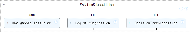
이제 학습을 완료했으니 score를 보자.
vc.score(X_train_scaled, Y_train), vc.score(X_test_scaled, Y_test)(0.9929577464788732, 0.986013986013986)학습이 99, 훈련이 98로 굉장히 잘맞췄다.
Y_test_pred=vc.predict(X_test_scaled)
print(classification_report(Y_test, Y_test_pred)) precision recall f1-score support
0 0.98 0.98 0.98 54
1 0.99 0.99 0.99 89
accuracy 0.99 143
macro avg 0.99 0.99 0.99 143
weighted avg 0.99 0.99 0.99 143조금이라도 더 높이고 싶으면, 최적화를 진행하며 그리드서치나 랜덤서치를 써서 하이퍼파라미터를 조절해야한다.
만약 hard로 진행한다면?
X_train, X_test, Y_train, Y_test=train_test_split(X,Y,random_state=42)
scaler=StandardScaler()
scaler.fit(X_train)
X_train_scaled=scaler.transform(X_train)
X_test_scaled=scaler.transform(X_test)
knn=KNeighborsClassifier()
lr=LogisticRegression()
dt=DecisionTreeClassifier()
vc=VotingClassifier(estimators=[("KNN",knn),("LR",lr),("DT",dt)], voting="hard")
vc.fit(X_train_scaled, Y_train)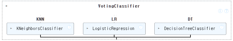
vc.score(X_train_scaled, Y_train), vc.score(X_test_scaled, Y_test)(0.9882629107981221, 0.993006993006993)그런데 이를보면, 테스트가 더 높게나왔다.
이런 경우에는 하이퍼파라미터를 찾아야하는 것이다.
꼭 hard나 soft 뭘 써야할지 정해져있는건 아니고 예측이 좋은걸 쓰면 된다.
사실 이번에는 서로 다른 알고리즘 3개를 사용했는데, 실제로는 하나의 알고리즘을 쓰는 경우가 많다.
3.1.3. DecisionTree
dt1=DecisionTreeClassifier(max_depth=5)
dt2=DecisionTreeClassifier(max_depth=3)
dt3=DecisionTreeClassifier(max_depth=5)
vc=VotingClassifier(estimators=[("DT1",dt1),("DT2",dt2),("DT3",dt3)], voting="hard")
vc.fit(X_train, Y_train)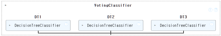
vc.score(X_train, Y_train), vc.score(X_test, Y_test)(0.9953051643192489, 0.958041958041958)Y_test_pred=vc.predict(X_test)
print(classification_report(Y_test, Y_test_pred)) precision recall f1-score support
0 0.93 0.96 0.95 54
1 0.98 0.96 0.97 89
accuracy 0.96 143
macro avg 0.95 0.96 0.96 143
weighted avg 0.96 0.96 0.96 143
이번에는 랜덤 서치를 넣어보자.
먼저 key, value를 어떻게 가져오는지 보자.
params_values={
"max_depth":randint(5,20),
"min_impurity_decrease":uniform(0.0001, 0.0006), # 0.0001과 0.0006 사이의 랜덤 실수 생성
"min_samples_split":randint(2,100)
}
params={}
for i in range(1,4):
for key,value in params_values.items(): # key, value 가져오기
params[f"DT{i}__{key}"]=value
params{'DT1__max_depth': <scipy.stats._distn_infrastructure.rv_discrete_frozen at 0x210a8aef700>,
'DT1__min_impurity_decrease': <scipy.stats._distn_infrastructure.rv_continuous_frozen at 0x210a8aeeda0>,
'DT1__min_samples_split': <scipy.stats._distn_infrastructure.rv_discrete_frozen at 0x210a8aeff10>,
'DT2__max_depth': <scipy.stats._distn_infrastructure.rv_discrete_frozen at 0x210a8aef700>,
'DT2__min_impurity_decrease': <scipy.stats._distn_infrastructure.rv_continuous_frozen at 0x210a8aeeda0>,
'DT2__min_samples_split': <scipy.stats._distn_infrastructure.rv_discrete_frozen at 0x210a8aeff10>,
'DT3__max_depth': <scipy.stats._distn_infrastructure.rv_discrete_frozen at 0x210a8aef700>,
'DT3__min_impurity_decrease': <scipy.stats._distn_infrastructure.rv_continuous_frozen at 0x210a8aeeda0>,
'DT3__min_samples_split': <scipy.stats._distn_infrastructure.rv_discrete_frozen at 0x210a8aeff10>}각 DT_키값의 형태로 가져오는 것을 알 수 있다.
따라서 estimator에서도 이 형식에 맞게 지정해주면 된다.
params_values={
"max_depth":randint(5,20),
"min_impurity_decrease":uniform(0.0001, 0.0006), # 0.0001과 0.0006 사이의 랜덤 실수 생성
"min_samples_split":randint(2,100)
}
params={}
for i in range(1,4):
for key,value in params_values.items(): # key, value 가져오기
params[f"DT{i}__{key}"]=value # __ 규칙
dt1=dt2=dt3=DecisionTreeClassifier()
vc=VotingClassifier(estimators=[("DT1",dt1),("DT2",dt2),("DT3",dt3)], voting="hard")
rs=RandomizedSearchCV(vc, params, n_iter=100, n_jobs=-1)
rs.fit(X_train,Y_train)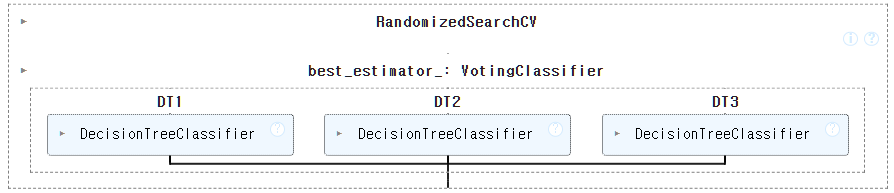
rs.score(X_train,Y_train), rs.score(X_test,Y_test)(0.9929577464788732, 0.951048951048951)전보다 더 떨어지는 결과가 나왔다.
이번에는 params를 각각 다르게 줘보자.
params={
"DT1__max_depth":randint(5,20),
"DT1__min_impurity_decrease":uniform(0.0001, 0.0006), # 0.0001과 0.0006 사이의 랜덤 실수 생성
"DT1__min_samples_split":randint(2,100),
"DT2__max_depth":randint(5,20),
"DT2__min_impurity_decrease":uniform(0.0001, 0.0006),
"DT2__min_samples_split":randint(2,100),
"DT3__max_depth":randint(5,20),
"DT3__min_impurity_decrease":uniform(0.0001, 0.0006),
"DT3__min_samples_split":randint(2,100)
}dt1=dt2=dt3=DecisionTreeClassifier()
vc=VotingClassifier(estimators=[("DT1",dt1),("DT2",dt2),("DT3",dt3)], voting="hard")
rs=RandomizedSearchCV(vc, params, n_iter=100, n_jobs=-1)
rs.fit(X_train,Y_train)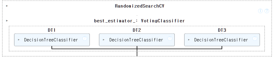
rs.score(X_train,Y_train), rs.score(X_test,Y_test)(0.9953051643192489, 0.9370629370629371)이도 별 차이 없다.
3.2. Bagging - RandomForest
Bagging, 샘플 데이터를 부트스트랩(복원추출) 방식
단일 경정 트리로 데이터 샘플링을 서로 다르게 가져가면서 학습 수행
대표적인 알고리즘: 랜덤포레스트
Voting은 각각 다르거나 같은 알고리즘을 가진 모델들이 하나의 큰 데이터를 동일하게 각각 가지고 진행했다면,
이 Bagging방식은 조금 다르다.
서로 다르거나 같은 알고리즘인데, 하나의 같은 데이터를 분할해서 가져간다.
이전 Validation, 검증 데이터가 cv=3으로 줬을때, 각각 겹치지 않게 가져갔던 것과 비슷하다.
그런데 이런 방식들 중에, 서로 다르지 않고 동일하게 모두 DecisionTree를 이용했더니 성능이 너무 좋았다.
이게 RandomForest다.
그래서 RandomForest에 디폴트로 DecisionTree가 100개가 들어있다.
그리고 이 RandomForest에 L1, L2규제를 준 것이 XGBoost다.
그런데 앞서 validation과 같이 겹치지 않게 뽑아가는 Bagging 방식인데,
랜덤포레스트처럼 디폴트가 100개라면 데이터를 다 따로따로 뽑을 수 없게된다.
그래서 부트스트랩 샘플(bootstrap smaple)이라는 것이 있다.
이는 데이터 세트에서 중복을 허용해서 데이터를 샘플링하는 것이다.
1000개의 샘플이 있다면, 먼저 1개를 뽑고, 뽑은 다음 다시 넣어서 그 다음 샘플을 뽑는 방식이다.
즉 1000개의 데이터 중에 100개를 만들어야 하니까 데이터가 부족해지고, 그를 방지하기 위해서
일부 뽑고 다시 집어넣어서 중복을 허용하는 것이다.
즉 동일한 데이터를 조합을 다르게 해서 무작위로 100개(default)를 것이다.
from sklearn.ensemble import RandomForestClassifier와인 데이터를 가져와서 사용한다.
wine=pd.read_csv("./data/wine.csv")
wine.shape(6497, 4)wine.head()| alcohol | sugar | pH | class | |
|---|---|---|---|---|
| 0 | 9.4 | 1.9 | 3.51 | 0.0 |
| 1 | 9.8 | 2.6 | 3.20 | 0.0 |
| 2 | 9.8 | 2.3 | 3.26 | 0.0 |
| 3 | 9.8 | 1.9 | 3.16 | 0.0 |
| 4 | 9.4 | 1.9 | 3.51 | 0.0 |
X=wine.iloc[:, :3]
Y=wine.iloc[:, -1]
X.shape, Y.shape
((6497, 3), (6497,))X_train, X_test, Y_train, Y_test=train_test_split(X,Y,test_size=0.2,random_state=42)
#forest=RandomForestClassifier(n_estimators=5, max_depth=5, n_jobs=-1, random_state=42)
forest=RandomForestClassifier(max_depth=5, n_jobs=-1, random_state=42)
forest.fit(X_train, Y_train)
scores=cross_validate(forest, X_train, Y_train, return_train_score=True, n_jobs=-1)n_estimators가 기본으로 100개인데 그렇게 많이 돌릴 필요 없으니 5개만 지정해주자.
랜덤포레스트에 DecisionTree가 5개가 들어가서 가지치기가 5가 된다.
print(scores["train_score"].mean())
print(scores["test_score"].mean())
0.8696363615536095
0.8608834308136523그러면 어떤 설명변수가 예측에 얼마나 영향을 미치는지 확인해보자.
forest.feature_importances_array([0.13104532, 0.63192419, 0.23703049])두번째인 와인이 가장 큰 영향을 미친 것을 알 수 있다.
Y_test_pred=forest.predict(X_test)
print(classification_report(Y_test, Y_test_pred))
precision recall f1-score support
0.0 0.76 0.60 0.67 341
1.0 0.87 0.93 0.90 959
accuracy 0.85 1300
macro avg 0.82 0.77 0.79 1300
weighted avg 0.84 0.85 0.84 1300이번에는 그냥 마음대로 정해줬는데 최적의 파라미터를 찾으러면
랜덤서치나 그리드 서치를 사용하면 된다.
3.3. GradientBoosting
여러개의 분류기가 순차적으로 학습하면서 앞에 학습한 분류기가 틀린 데이터에 대해서 가중치를 부여하면서 학습과 예측을 진행
자세한 설명은 설명이 잘 되어 있는 흠시 님의 Gradient Boost 글을 참고하자. https://dailyheumsi.tistory.com/116?category=877153
대표적 알고리즘: GBM, XGBoost, LightGBM, CatBoosting(최근)
from sklearn.ensemble import GradientBoostingClassifier# 예측평균 + (0.2 * 오차)
gb=GradientBoostingClassifier(n_estimators=500, learning_rate=0.2, random_state=42)
gb.fit(X_train, Y_train)
gb.score(X_train,Y_train), gb.score(X_test,Y_test)(0.9382335963055609, 0.8707692307692307)교차검증도 한번 해보자.
scores=cross_validate(gb, X_train, Y_train, return_train_score=True, n_jobs=-1)
print(scores["train_score"].mean())
print(scores["test_score"].mean())
0.9464595437171814
0.8780082549788999설명 변수의 특성 중요도는,
gb.feature_importances_array([0.15882696, 0.6799705 , 0.16120254])sugar다.
그러면 이런 GBM 알고리즘에 지금 가지치기를 안했기 때문에 과적합이 일어날 수 있다.
따라서 이런 과적합 방지를 위해 회귀에서 규제를 주는 것과 비슷한 방법이 있다.
#!pip install xgboost#!pip install lightgbmfrom xgboost import XGBClassifier
from lightgbm import LGBMClassifierL2 규제를 사용하는 XGBoost와 L1+L2 규제를 사용하는 LightGBM가 있다.
xg=XGBClassifier(n_estimators=500, random_state=42)
xg.fit(X_train, Y_train)
xg.score(X_train, Y_train), xg.score(X_test, Y_test)
(0.9940350202039638, 0.8676923076923077)이제 여기서 규제를 주려면, alpha값을 조절해주면 된다.
xg=XGBClassifier(n_estimators=500, random_state=42, reg_alpha=0.1)
xg.fit(X_train, Y_train)
xg.score(X_train, Y_train), xg.score(X_test, Y_test)
(0.9942274389070618, 0.8692307692307693)LightGBM도 다른게 없다.
lgb=LGBMClassifier(n_estimators=500)
xg.fit(X_train, Y_train)
xg.score(X_train, Y_train), xg.score(X_test, Y_test)
(0.9942274389070618, 0.8692307692307693)사실 이 XGBoost와 LightGBM은 잘 사용하지 않고, GBM만 잘 알아두면 된다.
그리고 이렇게 규제를 주는 릿지와 라쏘도 사실 많이 사용하지 않는다 아무리 조절해도 한계가 있다.
그냥 비선형 구조는 Tree를 가장 많이 사용한다.
평균과 오차와 가중치값을 줘서 곱하고 원래값과 빼서 줄여주는 GBM.