결측치(Missing Value)

• 이전 글에서 개념적으로 다루었던 내용이다.
  • 참고 링크 : [BDA 데이터분석전처리반(판다스)] 4주차 결측치
• 데이터셋에서 특정 값이 존재하지 않거나 누락된 상태를 의미

Sklearn 속 Imputer별 하이퍼파라미터 정리

IterativeImputer 주요 하이퍼파라미터

하이퍼파라미터	설명	가능한 값	기본값 (default)
estimator	누락값 추정에 사용할 추정기. 기본은 BayesianRidge, 다른 회귀 모델로 변경 가능	BayesianRidge, LinearRegression, KNeighborsRegressor 등	BayesianRidge()
max_iter	누락값 추정을 위한 최대 반복 횟수	정수	10
random_state	난수 생성기의 시드 값 설정. 동일한 결과 재현 가능	정수 또는 None	None
initial_strategy	초기 대치 전략	'mean', 'median', 'most_frequent', 'constant'	'mean'
imputation_order	특성을 대치하는 순서	'ascending', 'descending', 'roman', 'arabic', 'random'	'ascending'
skip_complete	완전한 케이스(누락값 없는 특성)를 계산에서 제외 여부	True, False	False
add_indicator	누락값 여부를 나타내는 지표 변수 추가 여부	True, False	False
tol	반복 중지 임계값. 이전과 현재 반복 사이 평균 제곱 차이가 작으면 중지	양수 실수	1e-3
n_nearest_features	각 특성을 대치할 때 사용할 다른 특성의 수. None이면 모든 특성을 사용	정수 또는 None	None
verbose	실행 중 출력 메시지의 양 제어	정수 (0 이상)	0
sample_posterior	BayesianRidge 추정기로 후방 분포에서 샘플링 여부	True, False	False

---

SimpleImputer 주요 하이퍼파라미터

하이퍼파라미터	설명	가능한 값	기본값 (default)
missing_values	누락값을 나타내는 placeholder	np.nan, 숫자 또는 기타 표현	np.nan
strategy	누락값 대체 전략	'mean', 'median', 'most_frequent', 'constant'	'mean'
fill_value	strategy="constant"일 때 사용할 대체 값	숫자, 문자열	Nㄱone
copy	True일 경우 원본 데이터 변경 없이 새 배열 생성	True, False	True
add_indicator	누락값 여부를 나타내는 지표 변수 추가 여부	True, False	False

---

KNNImputer 주요 하이퍼파라미터

하이퍼파라미터	설명	가능한 값	기본값 (default)
missing_values	누락값을 나타내는 placeholder	np.nan, 숫자 또는 기타 표현	np.nan
n_neighbors	누락값 대체에 사용할 가장 가까운 이웃의 수	정수	5
weights	이웃의 가중치 방식	'uniform', 'distance', 사용자 정의 함수	'uniform'
metric	거리 계산 메트릭	'nan_euclidean', 사용자 정의 거리 함수	'nan_euclidean'
copy	True일 경우 원본 데이터 변경 없이 새 배열 생성	True, False	True
add_indicator	누락값 여부를 나타내는 지표 변수 추가 여부	True, False	False

---

interpolate() 메서드 주요 옵션

옵션	설명	가능한 값
linear	기본값. 결측치를 양쪽 값으로부터 선형적으로 추정	'linear'
time	시간 간격을 고려하여 선형적으로 보간. 시계열 데이터에서 유용	'time'
index/values	인덱스 값에 기반하여 선형적으로 보간	'index', 'values'
pad/ffill	앞 방향으로 이전 유효 값으로 결측치 채움	'pad', 'ffill'
bfill/backfill	뒷 방향으로 다음 유효 값으로 결측치 채움	'bfill', 'backfill'
nearest	가장 가까운 인덱스 값으로 보간	'nearest'
polynomial	다항식 보간. order 옵션으로 다항식 차수 지정 필요	'polynomial', 정수 차수 (예: order=2)
slinear, quadratic, cubic	선형, 이차, 삼차 스플라인 보간	'slinear', 'quadratic', 'cubic'
akima	Akima의 3차 스플라인 보간법	'akima'
from_derivatives	데이터의 미분값을 알고 있을 때 이를 활용한 보간	'from_derivatives'

---

실습

결측치 처리

라이브러리 불러오기

import missingno as msno
from sklearn.experimental import enable_iterative_imputer
from sklearn.impute import IterativeImputer
import matplotlib.pyplot as plt
import pandas as pd
import seaborn as sns
import numpy as np

데이터 불러오기

import missingno as msno
from sklearn.experimental import enable_iterative_imputer
from sklearn.impute import IterativeImputer
import matplotlib.pyplot as plt
import pandas as pd
import seaborn as sns
import numpy as np

결측값 만들기

# 결측값 만들기
np.random.seed(42)

# 데이터 복사
data_with_missing = data.copy()

missing_rate = 0.05 # 결측치 퍼센트

# 전체 데이터에서 무작위로 결측값을 삽입할 위치 선택
n_total = data_with_missing.size
n_missing = int(n_total * missing_rate)

# 무작위 인덱스 생성
missing_indices = np.random.choice(n_total, n_missing, replace=False)

# 결측치 무작위로 만들기
rows, cols = np.unravel_index(missing_indices, data_with_missing.shape)
for row, col in zip(rows, cols):
  data_to_modify.iloc[row, col] = np.nan

data_with_missing.iloc[:, 1:] = data_to_modify

결측치 확인 (isna().sum())

data_with_missing.isna().sum()

	0
Year	11
Country	11
Spending_USD	17
Life_Expectancy	15

dtype: int64

결측치 확인 (msno.matrix())

msno.matrix(data_with_missing)
plt.show()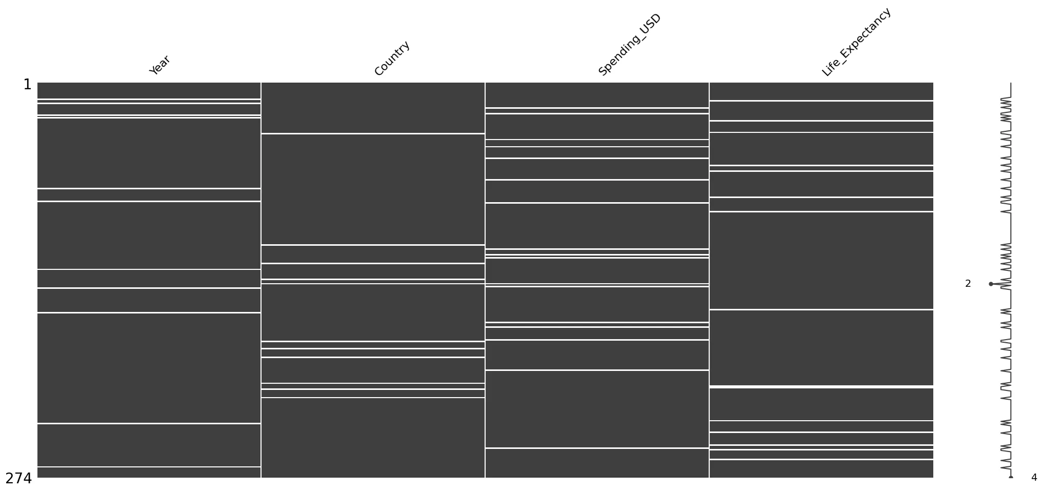

결측치 확인 (msno.bar())

msno.bar(data_with_missing)
plt.show()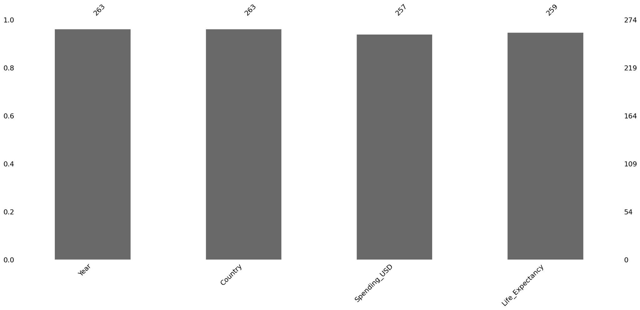

결측치 제거 (dropna())

data_with_missing.dropna(how='all')

Year	Country	Spending_USD	Life_Expectancy
0	1970	Germany	252.311
1	1970	France	192.143
2	1970	Great Britain	123.993
3	1970	Japan	150.437
4	1970	USA	326.961
...	...	...	...
269	2020	Germany	NaN
270	2020	France	5468.418
271	2020	Great Britain	5018.700
272	2020	Japan	4665.641
273	2020	USA	NaN

274 rows × 4 columns

• 삭제된 데이터가 없다.
  • how='all': 데이터가 거의 완전하지 않은 행/열만 삭제하고 싶을 때
  • how='any': 결측치가 하나라도 있으면 해당 행/열을 완전히 제거하고 싶을 때

결측치 대치 (fillna())

# 결측치 index 찾기
index = data_with_missing.index[data_with_missing.isna().any(axis=1)]

# 모두 0으로 대치
data_with_missing.iloc[index, :].fillna(0)

	Year	Country	Spending_USD	Life_Expectancy
11	0.0	Japan	185.390	73.2
12	1972.0	USA	397.097	0.0
14	0.0	Japan	205.778	73.4
17	1974.0	Japan	0.000	73.7
21	1975.0	Japan	0.000	74.3

# 평균값으로 대치
data_with_missing.iloc[index, :].fillna(data_with_missing['Life_Expectancy'].mean())

	Year	Country	Spending_USD	Life_Expectancy
11	77.887645	Japan	185.390000	73.200000
12	1972.000000	USA	397.097000	77.887645
14	77.887645	Japan	205.778000	73.400000
17	1974.000000	Japan	77.887645	73.700000
21	1975.000000	Japan	77.887645	74.300000

# 결측값을 뒤쪽 값으로 채우기
data_with_missing.fillna(method='bfill').head(5)

	Year	Country	Spending_USD	Life_Expectancy
0	1970.0	Germany	252.311	70.6
1	1970.0	France	192.143	72.2
2	1970.0	Great Britain	123.993	71.9
3	1970.0	Japan	150.437	72.0
4	1970.0	USA	326.961	70.9

결측치 처리에 따른 모델 성능 테스트

라이브러리 불러오기

from sklearn.model_selection import train_test_split
from sklearn.ensemble import RandomForestRegressor
from sklearn.metrics import mean_squared_error, r2_score
from sklearn.impute import KNNImputer

데이터 불러오기

data = sns.load_dataset("healthexp")

• 분석 목표 : 건강 지출과 연도, 국가가 기대수명(Life_Expectancy)에 미치는 영향을 분석하여 기대수명을 예측
  • 독립 변수 : Year, Country, Spending_USD
  • 종속 변수 : Life_Expectancy

결측값 만들기

np.random.seed(42)

data_with_missing = data.copy()

missing_rate = 0.1
n_missing = int(len(data_with_missing) * missing_rate)

missing_indices = np.random.choice(len(data_with_missing), n_missing, replace=False)

print("추가된 결측값 개수 : ", len(missing_indices))

data_with_missing.loc[missing_indices, 'Spending_USD'] = np.nan

• Spending_USD의 10% 정도를 임의로 결측치로 만듦

결측치 확인

data_with_missing.isna().sum()

	0
Year	0
Country	0
Spending_USD	27
Life_Expectancy	0

dtype: int64

결측치 처리 함수 정의

def drop_na(df, column):
    return df.dropna(subset=[column])

def mean_imputation(df, column):
    df_filled = df.copy()
    df_filled[column] = df_filled[column].fillna(df_filled[column].mean())
    return df_filled

def linear_interpolation(df, column):
    df_filled = df.copy()
    df_filled[column] = df_filled[column].interpolate(method='linear')
    return df_filled

def knn_imputation(df, column, n_neighbors=5):
    df_filled = df.copy()
    
    imputer = KNNImputer(n_neighbors=n_neighbors)
    df_filled[[column]] = imputer.fit_transform(df_filled[[column]])
  
    return df_filled

• drop_na : 결측값이 있는 행을 제거한다.
• mean_imputation : 결측값을 해당 열의 평균값으로 채운다.
• linear_interpolation : 결측값을 앞뒤 값으로 선형 보간법을 통해 채운다.
• knn_imputation : KNN 알고리즘을 사용하여 결측값을 가장 가까운 이웃의 값으로 채운다.

결측치 처리별 모델 학습 및 평가

column = 'Spending_USD'

for method_name, impute_func in methods.items():
    # 결측치 처리
    data_filled = impute_func(data_with_missing, column)

    # Feature와 Target 분리
    X = data_filled.drop(columns=column)
    y = data_filled[column]

    # 범주형 변수 더미 인코딩 (drop_first=True로 첫 번째 레벨 제거)
    X = pd.get_dummies(X, drop_first=True)

    # Train-Test Split
    X_train, X_test, y_train, y_test = train_test_split(X, y, test_size=0.2, random_state=42)

    # 모델 학습
    model = RandomForestRegressor(random_state=42)
    model.fit(X_train, y_train)

    # Train/Test 평가
    for dataset_name, X_data, y_data in (['Train', X_train, y_train], ['Test', X_test, y_test]):
        y_pred = model.predict(X_data)

        # 평가 지표 계산
        mse = mean_squared_error(y_data, y_pred)
        r2 = r2_score(y_data, y_pred)

        # 결과 저장
        result_now = pd.DataFrame({
            'Method': [method_name],
            'Dataset': [dataset_name],
            'MSE': [mse],
            'R2': [r2]
        })
        results = pd.concat([results, result_now], ignore_index=True)

# 결과 출력
print(results)

	Method	Dataset	MSE	R2
0	Drop NA	Train	1.008259e+04	0.997793
1	Drop NA	Test	7.043155e+04	0.985579
2	Mean Imputation	Train	1.184271e+04	0.997469
3	Mean Imputation	Test	3.112351e+06	-0.498801
4	Linear Interpolation	Train	1.184271e+04	0.997469
5	Linear Interpolation	Test	2.068646e+06	0.582370
6	Knn Imputation	Train	1.184271e+04	0.997469
7	Knn Imputation	Test	3.112351e+06	-0.498801

결과분석

• Drop NA: Train/Test 세트 모두 높은 R2, 낮은 MSE로 좋은 성능을 보인다.
• Mean Imputation & KNN Imputation: Train 세트에서는 높은 성능이지만, Test 세트에서는 R2 음수와 높은 MSE로 예측 실패하였다. 이는 결측치를 평균값으로 대체하거나, KNN 방식으로 대체해 데이터 왜곡이 발생했기 때문이다. (비정상적으로 낮음)
• Linear Interpolation: Train에서 좋은 성능, Test에서는 다소 성능 저하되지만 여전히 예측 가능하다.

결측치 처리 후 시각화

import matplotlib.pyplot as plt

fig, axes = plt.subplots(2,2, figsize=(16,12), sharex= True, sharey=True)
axes = axes.flatten()

for ax,(method_name, impute_func) in zip (axes, methods.items()):
    data_filled = impute_func(data_with_missing, column)

    ## 분포를 살펴보기
    sns.histplot(data_filled[column], bins= 30, kde=True, ax=ax)
    ax.set_title(f'Spending_USD Distribution - {method_name}')
    ax.set_xlabel('Spending_USD')
    ax.set_ylabel('Frequency')

plt.show()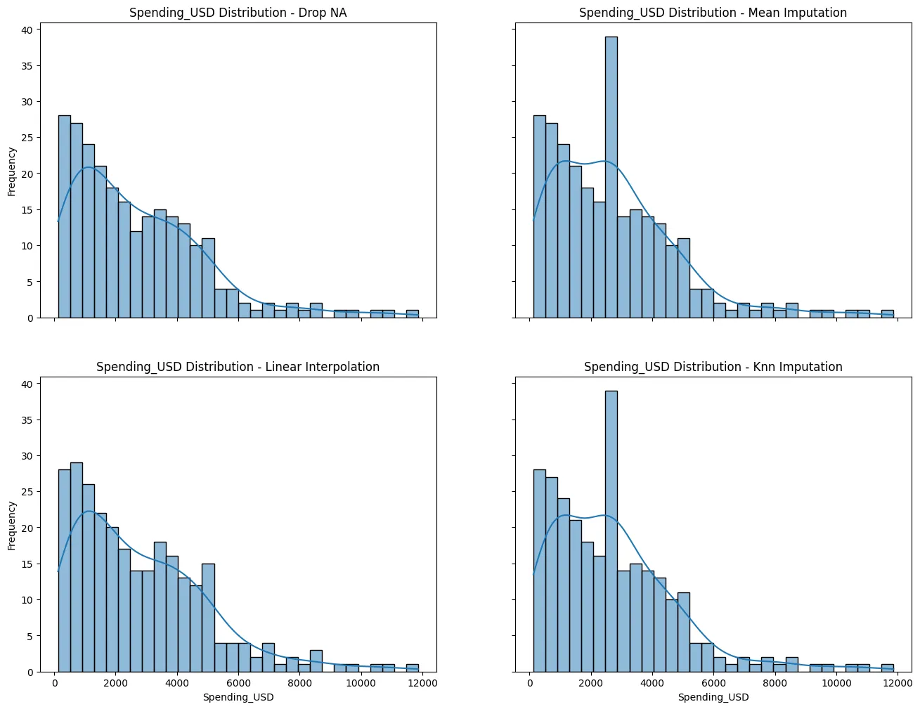

비정상적으로 낮은 점수 원인

• Mean Imputation & KNN Imputation: 특정 값에 집중된 데이터로 인해 모델이 과대적합(overfitting)되어 Test 세트에 일반화되지 못하였기 때문이다.

결론

• 현재 데이터셋에서는 결측치를 제거(Drop NA)하는 것이 분포를 덜 왜곡시키고, 모델의 성능도 더 안정적이기 때문에 다른 대체 기법(Mean, KNN 등)을 적용하는 것보다 더 나은 선택으로 보여진다.