Survival Analysis

• Survival analysis concerns a special kind of outcome variable : the time until an event occurs
• For example, suppose that we have conducted a five-year medical study, in which patients have been treated for cance
• We would like to fit a model to predict patient survival time, using features such as baseline health measurements or type of treatment
• Sounds like a regression problem. But there is an important complication : some of the patients have survived until the end of the study. Such a patient's survival time is said to be censored
• We do not wnat to discard this subset of surviving patients, since the fact that they survived at least five years amounts to valuable information

Non-medical Examples

• The applications of survival analysis extend far beyond medicine. For example, consider a company that wishes to model churn, the event when customers cancel subscription to a service
• The company might collect data on customers over some time period, in order to predict each customer's time to cancellation
• However, presumably not all customers will have cancelled their subscription by the end of this time period; for such customers, the time to cancellation is censored
• Survival analysis is a very well-studied topic within statistic. However, it has received relatively little attention in the machine learning community

Survival and Censoring Times

• For each individual, we suppose that there is a true failure or event time $T$, as well as a true censoring time $C$
• The survival time represents the time at which the event of interest occurs (such as death)
• By contrast, the censoring is the time at which censoring occurs: for example, the time at which the patient drops out of the study or the study ends

---

• We observe either the survival time $T$ or else the censoring time $C$. Specifically, we observe the random variable
  $Y=\min(T,C)$
• If the event occurs before censoring (i.e. $T<C$) then we observe the true survival time $T$; if censoring occurs before the event ($T>C$) then we observe the censoring time. We also observe a status indicator
  $\delta=\begin{cases}1\quad\text{if }T\leq C\\0\quad\text{if }T>C\end{cases}$
• Finally, in our dataset we observe $n$ paris $(Y,\delta)$, which we denote as $(y_1,\delta_1),\dots,(y_n,\delta_n)$

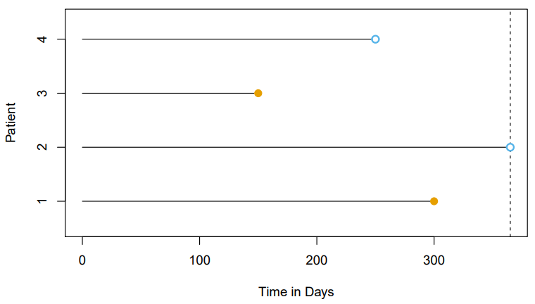
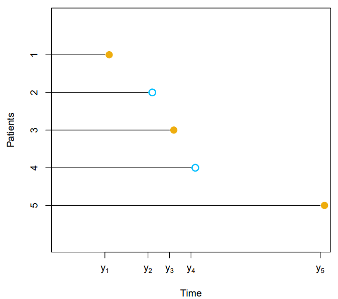
• Here is an illustration of censored survival data
• For patients $1$ and $3$, the event was observed
• Patient $2$ was alive when the study ended
• Patient $4$ dropped out of the study

A Closer Look at Censoring

• Suppose that a number of patients drop out of a cancer study early because they are very sick
• An analysis that does not take into consideration the reason why the patients dropped out will likely overestimate the true average survival time
• Similarly, suppose that males who are very sick are more likely to drop out of the study than females who are very sick
• Then a comparison of male and female survival times may wrongly suggest that males survive longer than females
• In general, we need to assume that, conditional on the features, the event time $T$ is independent of the censoring time $C$
• The two examples above violate the assumption of independent censoring

The Survival Curve

• The survival function ( or curve) is defined as
  $S(t)=\Pr(T>t)$
• This decreasing function quantifies the probability of surviving past time $t$
• For example, suppose that a company is interested in modeling customer churn
• Let $T$ represent the time that a customer cancels a subscription to the company's service
• Then $S(t)$ represents the probability that a customer cancels later than time $t$
• The larger the value of $S(t)$, the less likely that the customer will cancel before time $t$

Estimating the Survival Curve

• Consider the BrainCancer dataset, which contains the survival times for patients with primary brain tumors undergoing treatment with stereotactic radiation methods
• Only $53$ of the $88$ patients were still alive at the end of the study
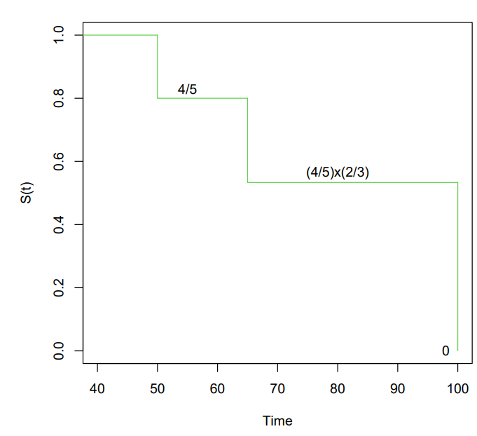
• Suppose we'd like to estimate $S(20)=\Pr(T>20)$, the probability that a patient survives for at least $20$ months
• It is tempting to simply compute the proportion of patients who are known to have survived past $20$ months, that is, the proportion of patients for whom $Y>20$
• This turns out to be $48/88$ or approximately $55\%$
• However, this does not seem quite right : $17$ of the $40$ patients who did not survive to $20$ months were actually censored, and this analysis implicitly assumes they died before $20$ months
• Hence it is probably an underestimate

Kaplen-Meier Survival Curve

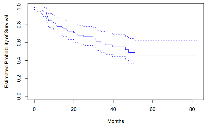
• Each point in the solid step-like curve shows the estimated probability of surviving past the time indicated on the horizontal axis
• The estimated probability of survival pas $20$ months is $71\%$, which is quite a bit higher than the naive estimate of $55\%$ presented earlier

The Log-Rank Test

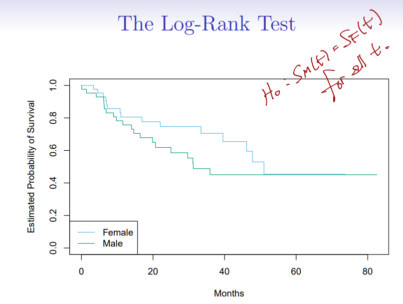
• We wish to compare the survival of males to that of females
• Shown are the Kaplan-Meier survival curves for the two groups
• Females seem to fare a little better up to about $50$ months, but then the two curves both level off to about $50\%$
• How can we carry out a formal test of equality of the two survival curves?
• At first glance, a two-sample $t$-test seems like an obvious choice : but the presence of censoring again creates a complication
• To overcome this challenge, we will conduct a log-rank test

---

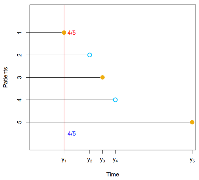
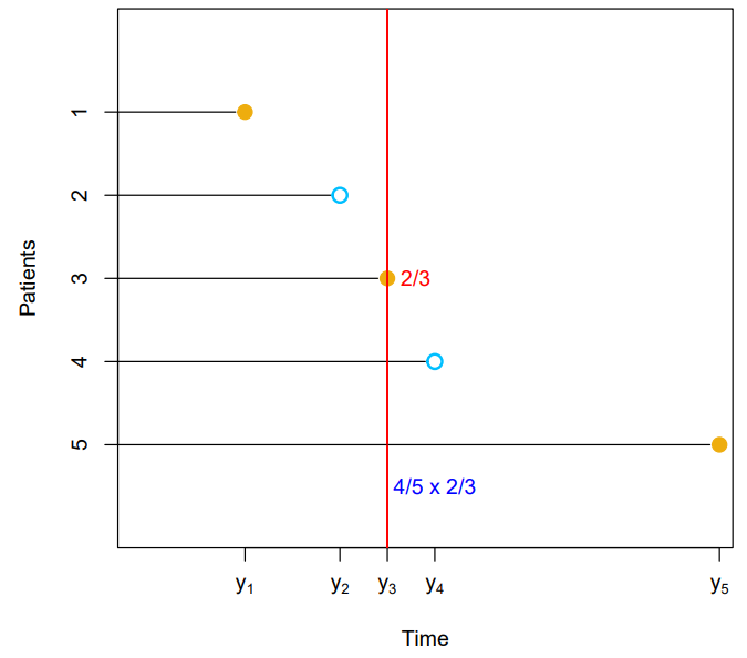
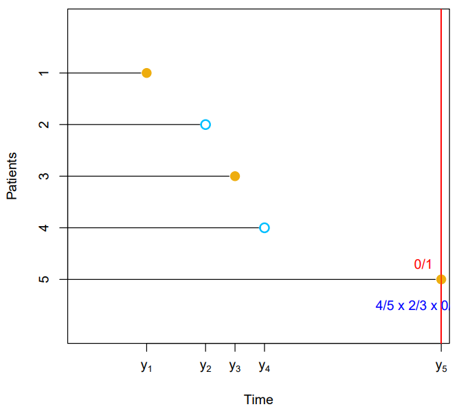
• Recall that $d_1<d_2<\cdots<d_K$ are the unique death times among the non-censored patients, $r_k$ is the number of patients at risk at time $d_k$, and $q_k$ is the number of patients who died at time $d_k$
• We further define $r_{1k}$ and $r_{2k}$ to be the number of patients in groups $1$ and $2$, respectively, who are at risk at time $d_k$
• Similarly, we define $q_{1k}$ and $q_{2k}$ to be the number of patients in groups $1$ and $2$, respectively, who died at time $d_k$
• Note that $r_{1k}+r_{2k}=r_k$ and $q_{1k}+q_{2k}=q_k$

Details of the Test Statistic

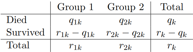
• At each death time $d_k$, we construct a $2\times 2$ table of counts of the form shown above
• Note that if the death times are unique (i.e. no two individuals die at the same time), then one of $q_{1k}$ and $q_{2k}$ equals one, and the other equals zero
• To test $\mathcal{H}_0:E(X)=0$ for some random variable $X$, one approach is to construct a test statistic of the form
  $W=\frac{X-E(X)}{\sqrt{\text{Var}(X)}}$
  where $E(X)$ and $\text{Var}(X)$ are the expectation and variance, respectively, of $X$ under $\mathcal{H}_0$
• In order to construct the log-rank test statistic, we compute a quantity that takes exactly the form above, with $X=\sum^K_{k=1}q_{1k}$, where $q_{1k}$ is given in the top left of the table above

---

• The resulting formula for the log-rank test statistic is
  $W=\frac{\sum^K_{k=1}(q_{1k}-E(q_{1k}))}{\sqrt{\sum^K_{k=1}\text{Var}(q_{1k})}}=\frac{\sum^K_{k=1}\left(q_{1k}-\frac{q_k}{r_k}r_{1k}\right)}{\sqrt{\sum^K_{k=1}\frac{q_k(r_{1k}/r_k)(1-r_{1k}/r_k)(r_k-q_k)}{r_k-1}}}$
• When the sample size is large, the log-rank test statistic $W$ has approximately a standard normal distribution
• This can be used to compute a $p$-value for the null hypothesis that there is no difference between the survival curves in the two groups

---

• Comparing the survival times of females and males on the BrainCancer data gives a log-rank test statistic of
  $W=1.2$
  which corresponds to a two-sided $p$-value of $0.2$
  Then, can not reject null hypothesis

Regression Models with a Survival Response

• We now consider the task of fitting a regression model to survival data
• We wish to predict the true survival time $T$
• Since the observed quantity $Y=\min(T,C)$ is positive and may have a long right tail, we might be tempted to fit a linear regression of $\log(Y)$ on $X$
• But censoring again creates a problem
• To overcome this difficulty, we instead make use of a sequential construction, similar to the idea used for the Kaplain-Meier survival curve

The Hazard Function

• The hazard function or hazard rate - also known as the force of mortality - is formally defined as
  $h(t)=\lim_{\Delta t\rightarrow 0}\frac{\Pr(t<T\leq t+\Delta t|T>t)}{\Delta t}$
  where $T$ is the (true) survival time
• It is the death rate in the instant after time $t$, given survival up to that time
• The hazard function is the basis for the Proportional Hazards Model

The Proportional Hazards Model

• The proportional hazards assumprion states that
  $h(t|x_i)=h_0(t)\exp\left(\sum^p_{j=1}x_{ij}\beta_j\right)$
  where $h_0(t)\geq 0$ is an unspecified function, known as the baseline hazard
• It is the hazrard function for an individual with features $x_{i1} = \cdots=x_{ip} = 0$
• The name proportional hazards arises from the fact that the hazard function for an individual with feature vector $x_i$ is some unknown function $h_0(t)$ times the factor
  $\exp\left(\sum^p_{j=1} x_{ij}\beta_j\right)$
• The quantity
  $\exp\left(\sum^p_{j=1}x_{ij}\beta_j\right)$
  is called the relative risk for the feature vector $x_i=(x_{i1},\cdots,x_{ip})$, realtive to that the feature vector $x_i=(0,\cdots,0)$
• What does it mean that the baseline hazard function $h_0(t)$ is unspecified
• Basically, we make no assumption about its functional form
• We allow the instantaneous probability of death at time $t$, given that one has survived at least until time $t$, to take any form
• This means that the hazard function is very flexible and can model a wide range of relationships between the covariates and survival time
• Our only assumption is that a one-unit increase in $x_{ij}$ corresponds to an increase in $h(t|x_i)$ by a factor of $\exp(\beta_j)$

---

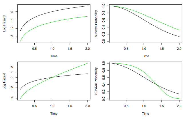
• Here is an example with $p=1$ and a binary covariate $x_i \in\{0,1\}$
• Top row : the log hazard and the survival function under the model are shown (green for $x_i=0$ and black for $x_i=1$). Because of the proportional hazards assumption, the log hazard functions differ by a constant, and the survival functions do not cross
• Bottom row : the proportional hazards assumptions does not hold

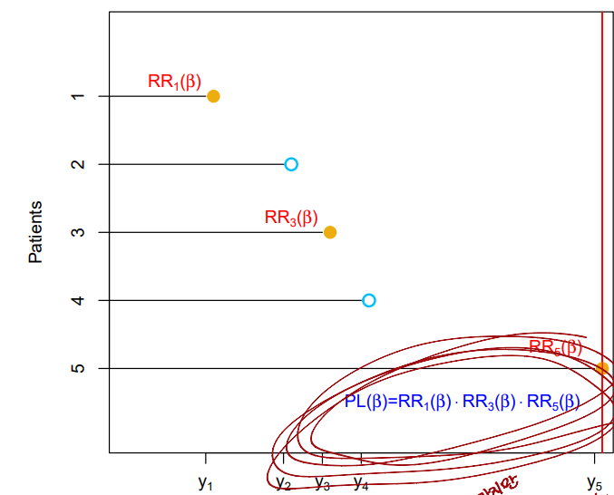
Partial Likelihood

• Because the form of the baseline hazard is unknown, we cannot simply plug $h(t|x_i)$ into the likelihood and then estimate $\beta=(\beta_1,\dots,\beta_p)^T$ by maximum likelihood
• The magic of Cox's proportional hazard model lies in the fact that it is in fact possible to estimate $\beta$ without having to specify the form of $h_0(t)$
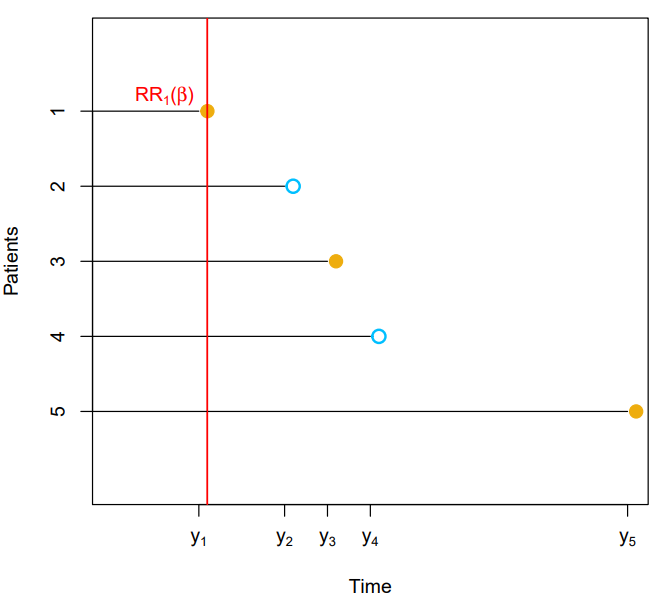
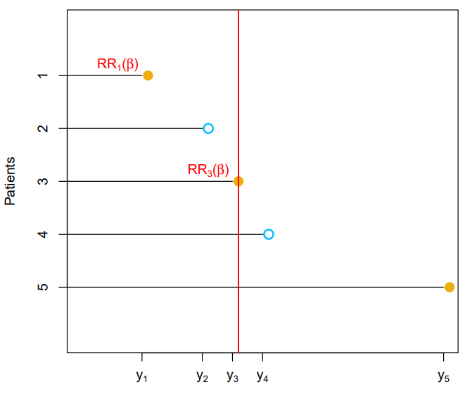
• To accomplish this, we make use of the same sequential in time logic that we used to derive the Kaplan-Meier survival curve and the log-rank test
• Then the total hazard at failure time $y_i$ for the at-risk observations is
  $\sum_{i':y_{i'}\geq y_i}h_0(y_i)\exp\left(\sum^p_{j=1}x_{i'j}\beta_j\right)$

---

• Therefore, the probability that the $i$th observation is the one to fail at time $y_i$ (as opposed to one of the other observations in the risk set) is
  $0\leq \frac{h_0(y_i)\exp\left(\sum^p_{j=1}x_{ij}\beta_j\right)}{\sum_{i':y_{i'}\geq y_i}h_0(y_i)\exp\left(\sum^p_{j=1}x_{i'j}\beta_j\right)}=\frac{\exp\left(\sum^p_{j=1}x_{ij}\beta_j\right)}{\sum_{i':y_{i'}\geq y_i}\exp\left(\sum^p_{j=1}x_{i 'j}\beta)_i\right)}\leq 1$
• Notice that the unspecified baseline hazard function $h_0(y_i)$ cancels out of the numerator and denominator

---

• The partial likelihood is simply the product of these probabilities over all of the uncensored observations
  $\text{PL}(\beta)=\prod_{i:\delta_i=1}\frac{\exp\left(\sum^p_{j=1}x_{ij}\beta_j\right)}{\sum_{i':y_{i'}\geq y_i}\exp\left(\sum^p_{j=1}x_{i'j}\beta_j\right)}$
• Critically, the partial likelihood is valid regardless of the true value of $h_0(t)$, making the model very flexible and robust
  

Relative Risk Functions at each Failure Time

All Contents written based on GIST - Machine Learning & Deep Learning Lesson(Instructor : Prof. sun-dong. Kim)