Moving Beyond Linearity
- Often the linearity assumption is good enough
- When its not...
- Polynomials
- Step functions
- Splines
- Local regression
- Generalized additive models
- Offer a lot of
flexibility, without losing the ease and interpretability of linear models
yi=β0+β1xi+β2xi2+⋯+βdxid+ϵi
Details
- Create new variables X1=X,X2=X2, etc and then treat as
multiple linear regression
- Not really interested in the coefficients; more interested in the fitted function values at any value x0
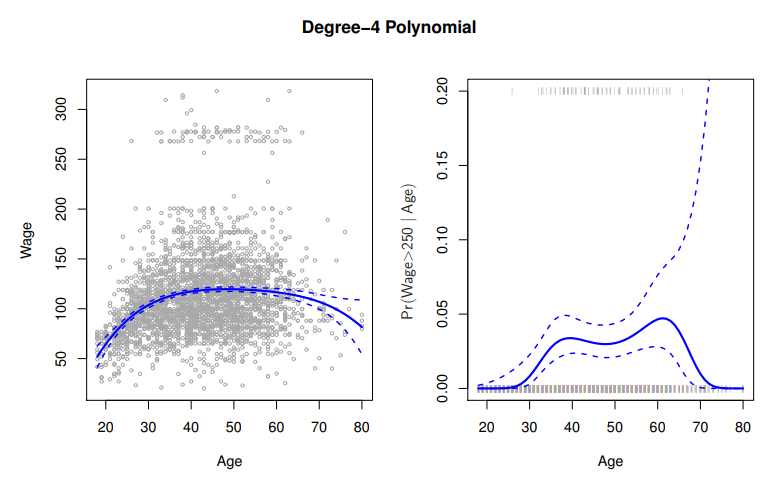
f^(x0)=β^0+β^1x0+β^2x02+β^3x03+β^4x04
- Since f^(x0) is a
linear function of the β^l, can get a simple expression for pointwise-variances Var[f^(x0)] at any value x0
- In the figure we have computed the fit and pointwise standard errors on a grid of values for x0
- We show f^(x0)±2×se[f^(x0)]
- We either fix the degree d at some reasonably
low value, else use cross-validation to choose d
Logistic Regression follows naturallyPr(yi>250∣xi)=1+exp(β0+β1xi+⋯+βdxid)exp(β0+β1xi+⋯+βdxid)
- To get
confidence intervals, compute upper and lower bounds on the logit scale, and then invert to get on probability scale
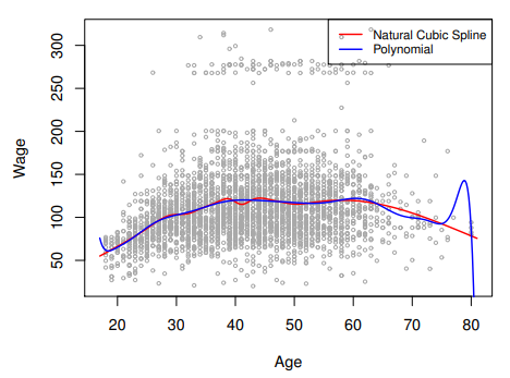
Polynomials have notorious tail behavior : very bad for extrapolation
- `Step Functions
C1(X)=I(X<35),C2(X)=I(35≤X<50)C3(X)=I(X≥65) 
- Useful way of creating interactions that are easy to interpret
- Interaction effect of Year and Age:
I(Year<2005)×Age,I(Year≥2005)×Age would allow for different linear functions in each age category
- Choice of
cutpoints or knots can be problematic
- For creating
nonlinearities, smoother alternatives such as splines are available
Picewise Polynomials
- Instead of a
single polynomial in X over its whole domain, we can rather use different polynomials in regions defined by knotsyi={β01+β11xi+β21xi2+β31xi3+ϵiβ02+β12xi+β22xi2+β32xi3+ϵiif xi<c,if xi≥c.
- Better to add
contraints to the polynomials e.g. continuity
Splines have the maximum amount of continuity

Linear Splines
- A
linear spline with knots at ξk, k=1,…,K is a piecewise linear polynomial continuous at each knot
- We can represent this model as
yi=β0+β1b1(xi)+β2b2(xi)+⋯+βK+1bK+1(xi)+ϵi, where the bk are basis functionsb1(xi)=xibk+1(xi)=(xi−ξk)+,k=1,…,K Here the ()+ means positive part(xi−ξk)+={xi−ξk0if xi>ξk,otherwise. 
Cubic Splines
- A
cubic spline with knots at ξk, k=1,…,K is a piecewise cubic polynomial with continuous derivatives up to order 2 at each knot
- Again we can represent this model with truncated
power basis functionsyi=β0+β1b1(xi)+β2b2(xi)+⋯+βK+3bK+3(xi)+ϵi,b1(xi)=xib2(xi)=xi2b3(xi)=xi3bk+3(xi)=(xi−ξk)+3,k=1,…,K where(xi−ξk)+3={(xi−ξk)30if xi>ξk,otherwise. 
Natural Cubic Splines
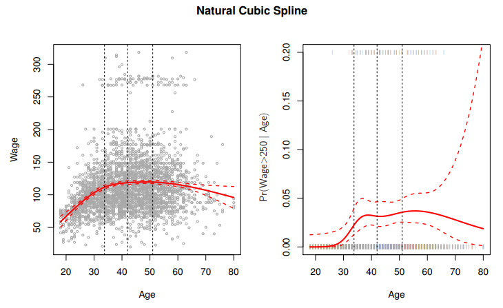
- A
natural cubic spline extrapolates linearly beyond the boundary knots
- This adds 4=2×2 extra contraints, and allows us to put more
internal knots for the same degrees of freedom as a regular cubic spline

Knot Placement
- One strategy is to decide K, the number of
knots, and then place them at appropriate quantiles of the observed X
- A
cubic spline with K knots has K+4 parameters or degrees of freedom
- A
natural spline with K knots has K degrees of freedom
Smoothing Splines
- Consider this criterion for fitting a smooth function g(x) to some data:
minimizeg∈Si=1∑n(yi−g(xi))2+λ∫(g′′(t))2dt
- The
first term is RSS, and tries to make g(x) match the data at each xi
- The
second term is a roughness penalty and controls how wiggly g(x) is
- It is modulated by the
tuning parameter λ≥0
- The
smaller λ, the more wiggly the function
- Eventually
interpolating yi when λ=0
- As λ→∞, the function g(x) becomes
linear
Some issues
- Smoothing splines avoid the
knot-selection issue, leaving a single λ to be chosen
- The vector of n fitted values can be written as g^λ=Sλy, where Sλ is a n×n matrix
- The
effective degrees of freedom are given bydfλ=i=1∑n{Sλ}ii.
Choosing lambda
- The
leave-one-out(LOO) cross-validation error is given byRSScv(λ)=i=1∑n(yi−g^λ(−i)(xi))2=i=1∑n[1−{Sλ}iiyi−g^λ(xi)]2. 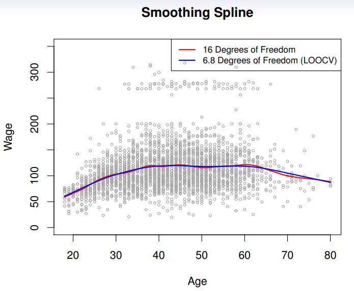
Local Regression
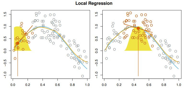
- With a sliding weight function, we fit seperate linear fits over the range of X by weighted least squares
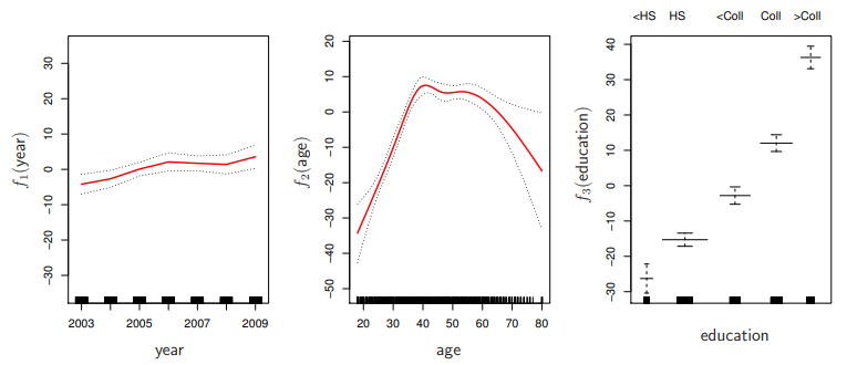
Generalized Additive Models
-
Allows for flexible nonlinearities in several variables, but retains the additive structure of linear models
yi=β0+f1(xi1)+f2(xi2)+⋯+fp(xip)+ϵi.
-
Can fit a GAM simply using, e.g. natural splines
lm(wage~ns(year,df=5) +ns(age, df = 5) + education)
- Coefficients not that interesting;
fitted functions are
- Can mix terms - some
linear, some nonlinear - and use anove() to compare models
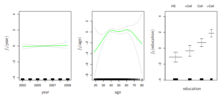
GAMs for Classification
log(1−p(X)p(X))=β0+f1(X1)+f2(X2)+⋯+fp(Xp).
All Contents written based on GIST - Machine Learning & Deep Learning Lesson(Instructor : Prof. sun-dong. Kim)
