Tree-based Methods

• Here we describe tree-based methods for regression and classification
• These involve stratifying or segmenting the predictor space into a number of simple regions
• Since the set of splitting rules used to segment the predictor space can be summarized in a tree, these types of approaches are known as decision-tree methods

Pros and Cons

• Tree-based methods are simple and useful for interpretation
• However they typically are not competitive with the best supervised learning approaches in terms of prediction accuracy
• Hence we also discuss bagging, random forests, and boosting
• Combining a large number of trees can often result in dramatic improvements in prediction accuracy, at the expense of some loss interpretation

The Basics of Decision Trees

• Decision trees can be applied to both regreesion and classification problems
• We first consider regression problems, and then move on to classification

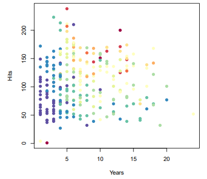
Baseball salary data : how would you stratify it?

• Salary is color-coded from low (blue, green) to high (yello, red)

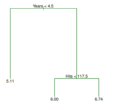
• The tree has two internal nodes and three terminal nodes, or leaves
• The number in each leaf is the mean of the response for the observations that fall there
• Overall, the tree stratifies or segments the players into three regions of predictor space
  $R_1=\{X|\text{Years}<4.5\}\\[0.3cm] R_2=\{X|\text{Years}\geq4.5,\text{Hits}<117.5\}\\[0.3cm] R_3=\{X|\text{Years}\geq 4.5,\text{Hits}\geq117.5\}$

Terminology for Trees

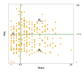
• In keeping with the tree analogy, the regions $R_1$,$R_2$ and $R_3$ are known as terminal nodes
• Decision trees are typically drawn upside down, in the sense that the leaves are at the bottom of the tere
• The points along the tree where the predictor space is split are referred to as internal nodes
• In the hitters tree, the two internal nodes are indicated by the text
  $\text{Years}<4.5$ and $\text{Hits}<117.5$

Interpretation of Results

• $\text{Years}$ is the most important factor in determining $\text{Salary}$ and players with less experience earn lower salaries than more experienced players
• Given that a player is less experienced, the number of $\text{Hits}$ that he made in the previous year seems to play little role in his $\text{Salary}$
• But among players who have been in the major leagues for five or more years, the number of $\text{Hits}$ made in the previous year does affect $\text{Salary}$, and players who made more $\text{Hits}$ last year tend to have higher salaries
• Surely an over-simplification, but compared to a regression model, it is easy to display, interpret and explain

Details of the tree-building process

1. We divide the predictor space - that is, the set of possible values for $X_1,X_2,\dots,X_p$ - into $J$ distinct and non-overlapping regions $R_1,R_2,\dots,R_J$
2. For every observation that falls into the region $R_j$, we make the same prediction which is simply the mean of the response values for the training observations in $R_j$

• In theory, the regions could have any shape,. However, we choose to divide the predictor space into high-dimensional rectangls, or boxes, for simplicity and for ease of interpretation of the resulting predictive model
• The goal is to find boxes $R_1,\dots,R_J$ that minimizes the RSS, given by
  $\sum_{j=1}^J\sum_{i\in R_j}(y_i-\hat y_{R_j})^2$
  where $\hat y_{R_j}$ is the mean response for the training observations within the $j$th box

---

• Unfortunately, it is computationally infeasible to consider every possible partition of the feature space info $J$ boxes
• For this reason, we take a top-down, greedy approach that is known as recursive binary splitting
• The approach is top-down because it begins at the top of the tree and then successively splits the predictor space
• Each split is indicated via two new branches further down on the tree
• It is greedy because at each step of the tree-building process, the best split is made at the particular step, rather than looking ahead and picking a split that will lead to a better tree in some future step

Greedy Approach of Tree-building Process

• We first select the predictor $X_j$ and the cutpoint $s$ such that splitting the predictor space into the regions
  $\{X|X_j<s\} \text{ and } \{X|X_j\geq s\}$
  leads to the greatest possible reduction in RSS
• Next, we repeat the process, looking for the best predictor and best cutpoint in order to split the data further so as to minimize the RSS within each of the resulting regions
• However, this time, instead of splitting the entire predictor space, we split one of the two previously identified regions
• Again, we look to split one of these regions further, so as to minimize the RSS. The process continues until a stopping criterion is reached

  For instance, we may continue until no region contains more than five observations

Predictions

• We predict the response for a given test observation using the mean of the training observations in the region to which that test observation belongs
• A five-region example of this approach is shown in the next
  
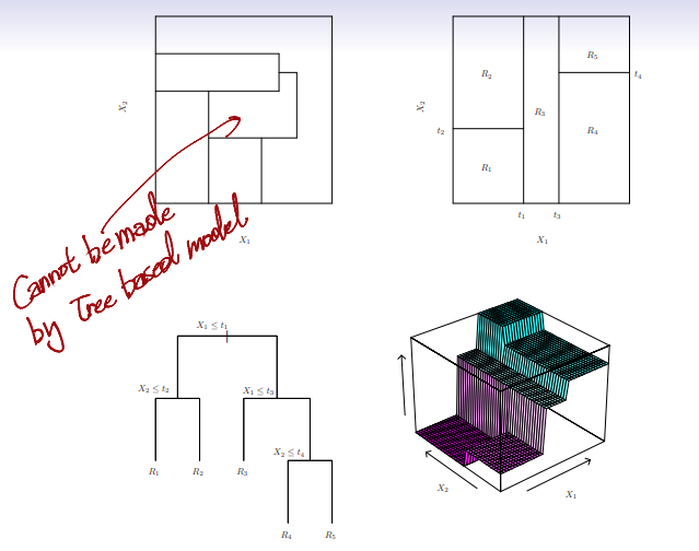
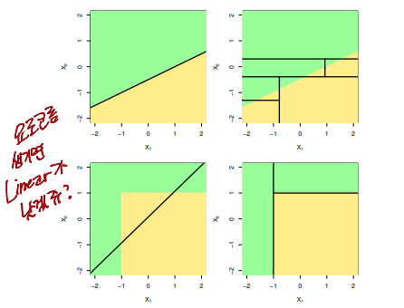
  • Top Left : A partition of two-dimensional feature space that could not result from recursive binary splitting
  • Top Right : The output of recursive binary splitting on a two-dimensional example
  • Bottom Left : A tree corresponding to the partition in the top right pannel
  • Bottom Right : A perspective plot of the prediction surface corresponding to that tree

Pruning a tree

• The process described above may produce good predictions on the training set, but is likely to overfit the data, leading to poor test set perfomance
• A smaller tree with fewer splits (that is, fewer regions $R_1,\dots,R_J$) might lead to lower variance and better interpretation at the cost of little bias
• One possible alternative to the process described above is to grow the tree only so long as the decrease in the RSS due to each split exceeds some (high) threshold
• This strategy will result in smaller trees, but is too short-sighted

  a seemingly worthless split early on in the tree might be followed by a very good split - that is, a split that leads to a large reduction in RSS later on

---

• A better strategy is to grow a very large tree $T_0$, and then prune it back in order to obtain a subtree
• Cost complexity pruning - also known as weakest link pruning - is used to do this
• We consider a sequence of trees indexed by a nonnegative tuning parameter $\alpha$
• For each value of $\alpha$ there corresponds a subtree $T\in T_0$ such that
  $\sum_{m=1}^{|T|}\sum_{i:x_i\in R_m}(y_i-\hat y_{R_m})^2+\alpha|T|$
  • RSS : $\sum_{m=1}^{|T|}\sum_{i:x_i\in R_m}(y_i-\hat y_{R_m})^2$
  • Number of Terminal Node : $|T|$
• Here $|T|$ indicates the number of terminal nodes of the Tree $T,R_m$ is the rectangle(i.e. the subset of predictor space) corresponding to the $m$th terminal node, and $\hat y_{R_m}$ is the mean of the trainin observations in $R_m$

Choosing the best subtree

• The tuning parameter $\alpha$ controls a trade-off between the subtree's complexity and its fit to the training data
• We select an optimal value $\hat \alpha$ using cross-validation
• We then return to the full data set and obtain the subtree corresponding to $\hat \alpha$

---

Summary : tree algorithm

1. Use recursive binary splitting to grow a large tree on the training data, stopping only when each terminal node has fewer than some minimum number of observations
2. Apply cost complexity pruning to the large tree in order to obtain a sequence of best subtrees, as a function of $\alpha$
3. Use $K$-fold cross-validation to choose $\alpha$. For each $k=1,\dots,K$
   1. Repeat Steps 1 and 2 on the $\frac{K-1}{K}$th fraction of the training data, excluding the $k$th fold
   2. Evaluate the mean squared prediction error on the data in the left-out $k$th fold, as a function of $\alpha$
4. Return the subtree from Step 2 that corresponds to the chosen value of $\alpha$
   

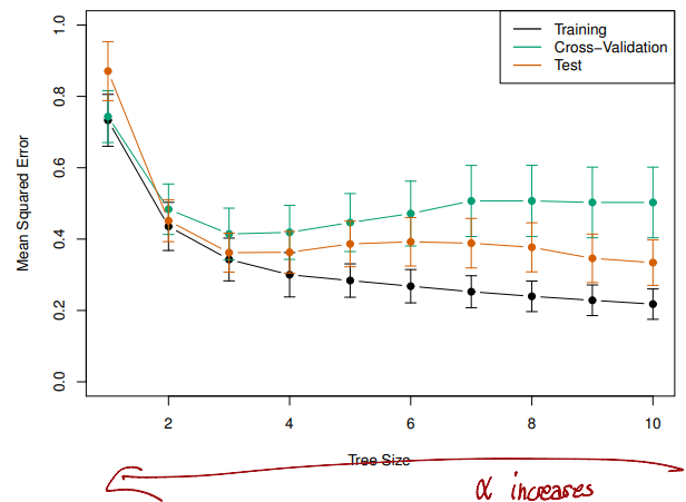
   Then we could pick $\alpha$ value when the Tree Size has become 3 using 1 std rule

Classification Trees

• Very similar to a regression tree, except that it is used to predict a qualitative response rather than a quantitative one
• For a classification tree, we predict that each observation belongs to the most commonly occurring class of training observations in the region to which it belongs
• Just as in the regression setting, we use recursive binary splitting to grow a classification tree
• In the classification setting, RSS cannot be used as a criterion for for making the binary splits

---

• A natural alternative to RSS is the classification error rate
  $E=1-\max_k(\hat p_{mk})$
  Here $\hat p_{mk}$ represents the proportion of training observations in the $m$th region that are from the $k$th class.
• However classification error is not sufficiently sensitive for tree-growing, and in practice two other measures are preferable

Gini index and Deviance

• The Gini index is defined by
  $G=\sum_{k=1}^K \hat p_{mk}(1 - \hat p_{mk})$
• For this reason the Gini index is referred to as a measure of node purity - a small value indicates that a node contains predominantly observations from a single class
• An alternative to the Gini index is cross-entropy, given by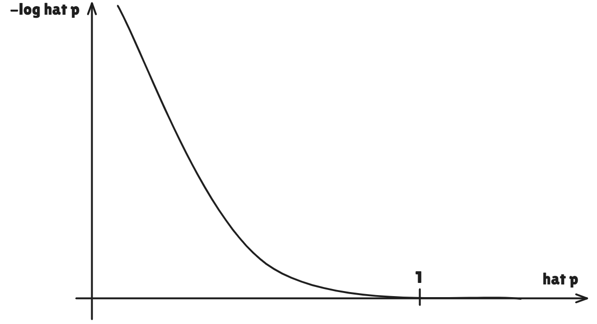
  $D=-\sum_{k=1}^K \hat p_{mk}\log \hat p_{mk}$
  
• It turns out that the Gini index and the cross-entropy are very similar numerically

Trees Versus Linear Models

• Top Row : True linear boundary
• Bottom Row : true non-linear boundary
• Left Column : Linear model
• Right Column : non-linear model

Advantages and Disadvantages of Trees

• Advantages
  • Trees are very easy to explain to people. They are even easier to explain than linear regression
  • Some people believe that decision trees more closely mirror human decision-making than do the regression and classification approaches seen in previous chapters
  • Trees can be displayed graphically and are easily interpreted even by a non-expert
  • Trees can easily handle qualitative predictors without the need to create dummy variables
• Disadvantages
  • Unfortunately, trees generally do not have the same level of predictive accuracy as some of the other regression and classification approaches seen in this book

---

Bagging

• Bootstrap aggregation, or bagging, is a general-purpose procedure for reducing the variance of a statistical learning method
• Recall that given a set of $n$ independent observations $Z_1,\dots,Z_n$, each with variance $\sigma^2$ the variance of the mean $\bar Z$ of the observations is given by $\sigma^2/n$
• In other words, averaging a set of observations reduces variance
• Of course, this is not practical because we generally do not have access to multiple training sets
• Instead, we can bootstrap, by taking repeated samples from the (single) training data set
• In this approach we generate $B$ different bootstrapped training data sets
• We train our method on the $b$th bootstrapped training set in order to get $\hat f^{*b}(x)$, the prediction at a point $x$
• We then average all the predictions to obtain
  $\hat f_{\text{bag}}(x)=\frac{1}{B}\sum_{b=1}^B\hat f^{*b}(x)$

  This is called bagging

Bagging classification trees

• The above prescription applied to regression trees
• For classification trees : for each test observation, we record the class predicted by each of the $B$ trees, and take a majority vote
  
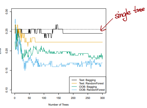
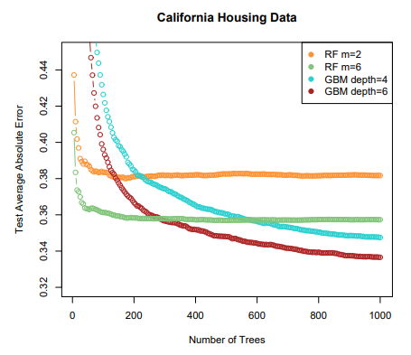
  • The test error (black and orange) is shown as a function of $B$, the number of bootstrapped training sets used
  • Random forests were applied with $m=\sqrt p$
  • The dashed line indicates the test error resulting from a single classificaion tree
  • The green and blue traces show the OOB error, which in this case is considerably lower

Out-of-Bag Error Estimation

• It turns out that there is a very straightforward way to estimate the test error of a bagged model
• Recall that the key to bagging is that trees are repeatedly fit to bootstrapped subsets of the observations
• One can show that on average, each bagged tree makes use of around two-thirds of the observations
• The remaining one-third of the observations not used to fit a given bagged tree and referred to as the out-of-bag (OOB) observations
• We can predict the response for the $i$th observation using each of the trees in which that observation was OOB
• This will yield aroung $B/3$ predictions for the $i$th observation, which we average
• This estimate is essentially the LOO cross-validation error for bagging, if $B$ is large

Random Forests

• Random forests provide an improvement over bagged trees by way of a small tweak that decorrelates the trees
• This reduces the variance when we average the trees
• As in bagging, we build a number of decision trees on bootstrapped training samples
• But when building these decision trees, each time a split in a tree is considered, a random selection of $m$ predictors is chosen as split candidates from the full set of $p$ predictors
• The split is allowed to use only one of those $m$ predictors
• A fresh selection of $m$ predictors is taken at each split, and typically we choose $m\approx\sqrt p$
  That is, the number of predictors considered at each split is approximately equal to the square root of the total number of prdictors

Boosting

• Like bagging, boosting is a general approach that can be applied to many statistical learning methods for regression or classification
• We only discuss boosting for decision trees
• Recall that bagging involves creating multiple copies of the original training data set using the bootstrap, fitting a seperate decision tree to each copy, and then combining all of the trees in order to create a single predictive model
• Notably, each tree is built on a bootstrap data set, independent of the other trees
• Boosting works in a similar way, except that the trees are grown sequentially

Boosting algorithm for regression trees

1. Set $\hat f(x)=0$ and $r_i=y_i$ for all $i$ in the training set
2. For $b=1,2,\dots,B$, repeat :
   1. Fit a tree $\hat f^b$ with $d$ splits $(d+1)$ terminal nodes to the training data $(X,r)$
   2. Update $\hat f$ by adding in a shrunken version of the new tree :
      $\hat f(x)\leftarrow\hat f(x)+\lambda\hat f^b(x)$
   3. Update the residuals
      $r_i\leftarrow r_i-\lambda\hat f^b(x_i)$
3. Output the boosted model
   $\hat f(x)=\sum_{b=1}^B\lambda\hat f^b(x)$

What is the idea behind this procedure?

• Unlike fitting a single large decision tree to the data, which amounts to fitting the data hard and potentially overfitting, the boosting approach instead learns slowly
• Given the current model, we fit a decision tree to the residual from the model
• We then add this new decision tree into the fitted function in order to update the residuals
• Each of these trees can be rather small, with just a few terminal nodes, determined by the parameter $d$ in the algorithm
• By fitting small trees to the residuals, we slowly improve $\hat f$ in areas where it does not perform well
• The shrinkage parameter $\lambda$ slows the process down even further, allowing more and different shaped trees to attack the residuals

Boosting for classification

• Boosting for classification is similar in spirit to boosting for regression, but is a bit more complex
• We will not go into detail here, nor do we in the text book
• Students can learn about the details in Elements of Statistical Learning, chapter 10

Tuning parameters for boosting

1. The number of trees $B$
   Unlike bagging and random forests, boosting can overfit if $B$ is too large, although this overfitting tends to occur slowly if at all. We use cross-validation to select $B$
2. The shrinkage parameter $\lambda$
   A small positive number. This controls the rate at which boosting learns. Typical values are 0.01 or 0.001, and the right choice can depend on the problem.
   Very small $\lambda$ can require using a very large value of $B$ in order to achieve good performance
3. The number of splits $d$
   In each tree, which controls the complexity of the boosted ensemble
   Often $d=1$ works well, in which case each tree is a stump, consisting of a sinple split and resulting in an additive model.
   More generally $d$ is the interaction depth, and controls the interaction order of the boosted model, since $d$ splits can involve at most $d$ variables
   

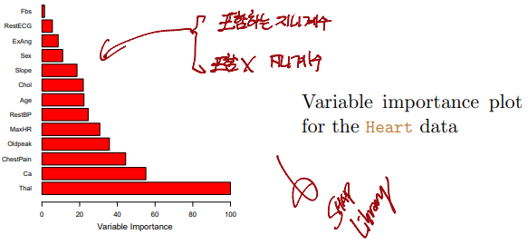
Variable importance measure

• For bagged/RF regression trees, we record the total amount that the RSS is decreased due to splits over a given predictor, averaged over all $B$ trees
• A large value indicates an important predictor
• Similarly, for bagged/RF classification trees, we add up the total amount that the Gini index is decreased by splits over a given predictor, averaged over all $B$ trees
  

All Contents written based on GIST - Machine Learning & Deep Learning Lesson(Instructor : Prof. sun-dong. Kim)