Multiple Hypothesis Testing
- This session focuses on
multiple hypothesis testing - A single null hypothesis might look like
: the expected blood pressures of mice in the control and treatment groups are the same
- We will now consider testing null hypotheses,
where e.g.: the expected values of the biomarker among mice in the control and treatment groups are equal
- In this setting, we need to be careful to avoid incorrectly rejecting too many null hypotheses,
i.e. having too many false positives
A Quick Review of Hypothesis Testing
- Hypothesis tests allow us to answer simple
yes-or-noquestions, such as- Is the true coefficient in a linear regression equal to zero?
- Does the expected blood pressure among mice in the treatment group equal the expected blood pressure among mice in the control group?
- Hypothesis testing proceeds as follows :
- Define the null and alternative hypotheses
- Construct the test statistic
- Compute the -value
- Decide whether to reject the null hypothesis
1. Define the Null and Alternative Hypotheses
- We divide the world into
nullandalternativehypotheses - The
null hypothesis, is the default state of belief about the world. For instance :- The true coefficient equals
zero - There is no difference in the expected blood pressure
- The true coefficient equals
- The
alternative hypothesis, represents something different and unexpected. For instnace :- The true coefficient is
non-zero - There is a difference in the expected blood pressure
- The true coefficient is
2. Construct the Test Statistic
- The test statistis summarizes the extent to which our data are consistent with
- Let respectively denote the average blood pressure for the mice in the treatment and control groups
- To test : , we use a two-sample -statistic
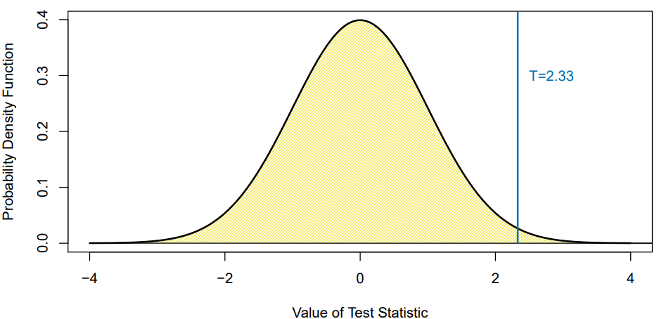
3. Compute the p-value
- The -value is the probability of observing a test statistic at least as extreme as the observed statistic,
under the assumption thatis true - A small -value provides evidence
against - Suppose we compute for our test of
- Under for a two-sample -statistic
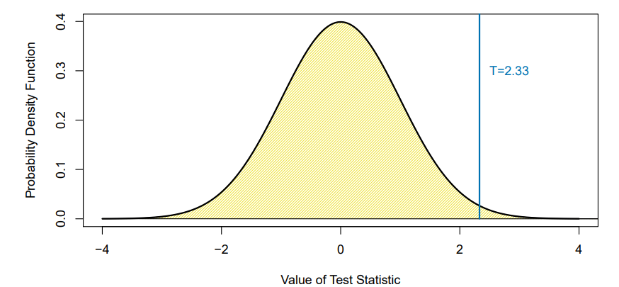
- The p-value is because, if is true, we would only see this large of the time
4. Decide Whether to Reject Null Hypothesis, Part 1
- A small -value indicates that such a large value of the test statistic is unlikely to occur under
- So, a small -value provides evidence against
- If the -value is sufficiently small, then we will want to
reject - But how small is small enough? To answer this, we need to understand the
Type 1 Error
4. Decide Whether to Reject Null Hypothesis, Part 2
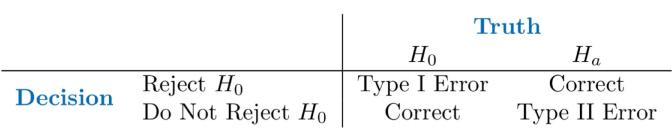
- The
Type 1 Error rateis the probability of making aType 1 Error - We want to ensure a small
Type 1 Error rate - If we reject when the p-value is less then , then the
Type 1 Error ratewill be at most - So, we reject when the p-value falls below some : often we choose to equal or
Multiple Testing
- Now suppose that we wish to test
null hypotheses, - Can we simply reject all
null hypothesesfor which the corresponding -value falls below - If we reject all null hypotheses for which the -value falls below , then how many
Type 1 Errorwill be make?
A Thought Experiment
- Suppose that we flip a fair coin ten times, and we wish to test
- We'll probably get approximately the same number of heads and tails
- The -value probably won't be small. We do not reject
- But what if we flip fair coins ten times each?
- We'd except one coin (on average) to come up all tails
- The -values for the
null hypothesisthat this particular coin is fair is less than ! - So we would conclude it is not fair, i.e. we
reject null hypothesis, even though it's a fair coin
- If we test a lot of hypotheses, we are almost certain to get one very small -value by chance
The Challenge of Multiple Testing
- Suppose we test , all of which are true, and reject any
null hypothesiswith a -value below - Then we except to falsely reject approximately
null hypotheses - If , then we expect to falsely reject
null hypothesesby chance!That's a lot of Type 1 Errors, i.e. false positives
The Family-Wise Error Rate
- The
family-wise error rate(FWER) is the probability of makingat least oneType 1 error when conducting hypothesis tests
Challenges in Controlloing the FWER
- If the tests are
independentand all are true then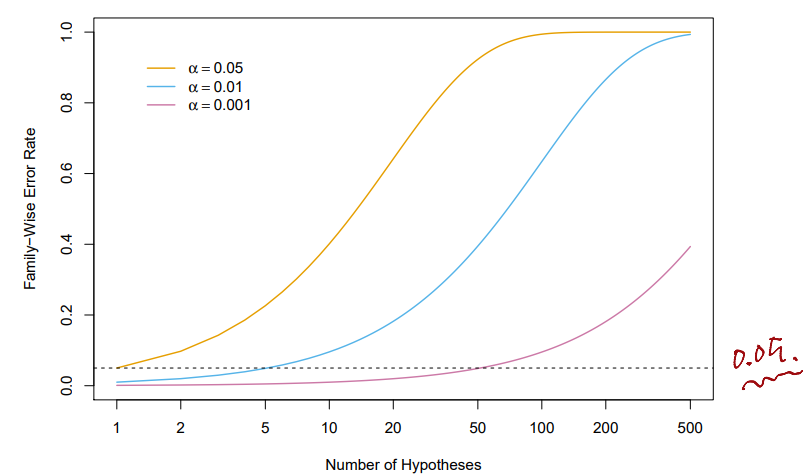
The Bonferroni Correction
- Where is the event that we
falsely rejectthe thnull hypothesis - If we only reject hypotheses when the -value is less than , then
- This is the
Bonferroni Correction: to controlFWERat level , reject anynull hypothesiswith -value below
Holm's Method for Controlling the FWER
- Compute -values, for the
null hypotheses - Order the -values so that
- Define
- Reject all
null hypotesesfor which- Holm's method controls the
FWERat level
- Holm's method controls the
Holm's Method on the Fund Manager Data
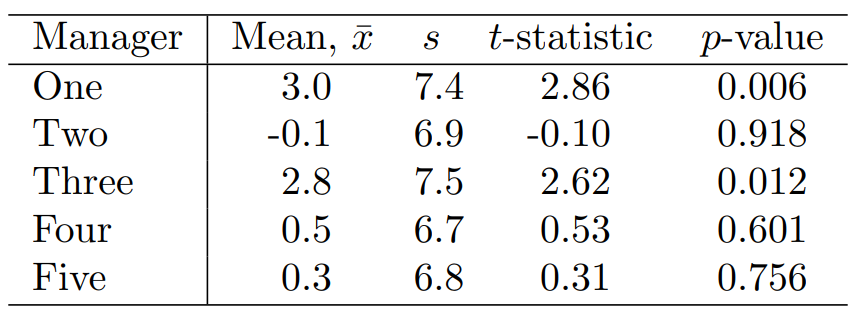
- The ordered -values are
- The
Holm procedurerejects the first twonull hypotheses, because Holmrejects for thefirstandthirdmanagers, butBonferronionly rejects for thefirstmanager
Comparison with m=10 p-values
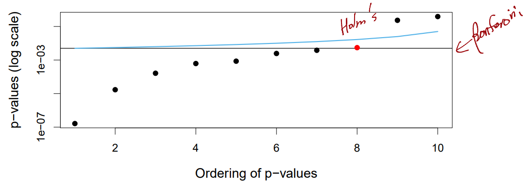
- Aim to control
FWERat - -values below the balck horizontal line are rejected by
Bonferroni - -values below the blue line are rejected by
Holm HolmandBonferronimake the same conclusion on the black points, but onlyHolmrejects for the red point
A More Extreme Example
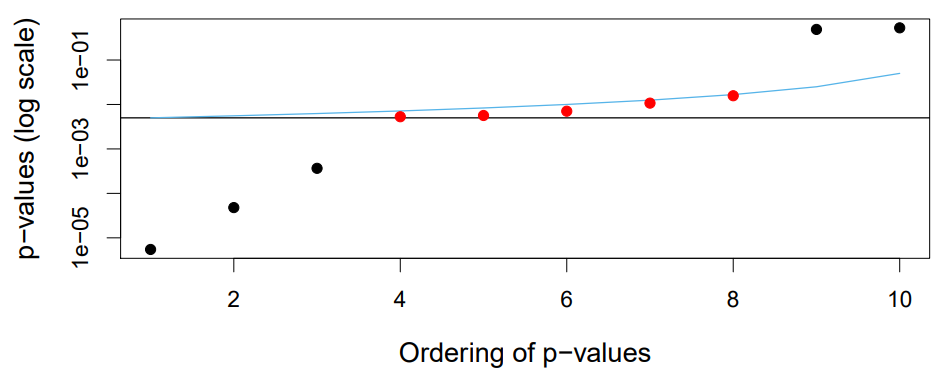
- Now five hypotheses are rejected by
Holmbut not byBonferroni... - even though both control
FWERat
Holm or Bonferroni?
Bonferroniis simple : reject anynull hypothesiswith a -value belowHolmis slightly more complicated, but it will lead to more rejections while controllingFWERSo,
Holmis a better choice
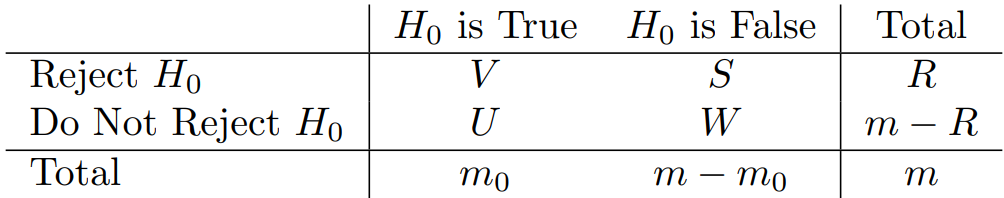
The False Discovery Rate
- Back to this table :
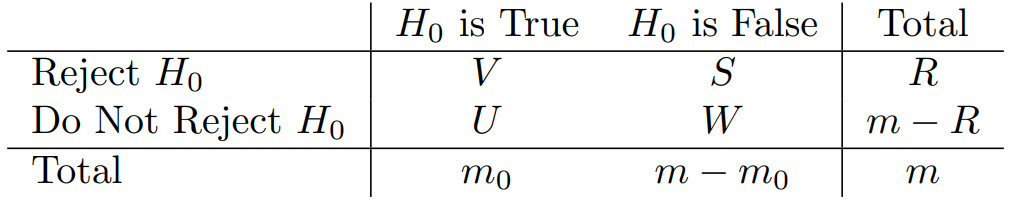
- The
FWERrate focuses on controlling , i.e., the probability of falsely rejectinganynull hypothesis - This is a tough ask when is large. It will cause us to be super conservative(i.e. to very rarely reject)
- Instead, we can control the
false discovery rate
Intuition Behind the False Discovery Rate
- A scientist conducts a hypothesis test on each of drug candidates
- She wants to identify a smaller set of promising candidates to investigate further
- She wants reassurance that this smaller set is really
promising, i.e. not too many falsely rejected 's FWERcontrolsFDRcontrols the fraction of candidates in the smaller set that are really false rejections.
Benjamini-Hochberg Procedure to Control FDR
- Specify , the level at which to control the
FDR - Compute -values for the
null hypotheses - Order the -values so that
- Define
- Reject all null hypotheses for which
Then,FDR
A Comparison of FDR vs FWER
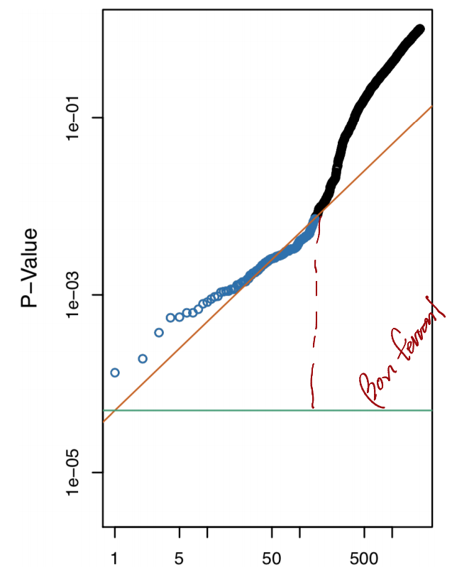
- Here, -values for
null hypothesesare displayed - To control
FWERat level withBonferroni: reject hypotheses below green line - To control
FDRat level withBenjamini-Hochberg: reject hypothese shown in blue
- Consider p-values from the Fund data :
- To control
FDRat level usingBenjamini-Hochberg:- Notice that
- So, we reject and
- To control
FWERat level usingBonferroni:- We reject any
null hypothesisfor which the -value is less than - So, we reject only
- We reject any
Re-Sampling Approaches
- So far, we have assumed that we want to test some
null hypothesiswith some test statistic , and that we know the distribution of under - This allows us to compute the -value
- What if this theoretical null distribution is unknown?
A Re-Sampling Approach for a Two-Sample t-Test
- Suppose we want to test versus , using independent observations from and independent observations from
- The two-sample -statistic takes the form
- If and are large, then approximately follows a distribution under
- If and are small, then we don't know the theorectical null distribution of
- Let's take a
permutationorre-samplingapproach...
- Compute the two-sample -statistic on the original data and
- For (where is a large number, like ) :
2.1.Randomly shufflethe observations
2.2. Call the first shuffled observations and call the remaining observations
2.3. Compute a two-sample -statistic on the shuffled data, and call it - The -value is given by
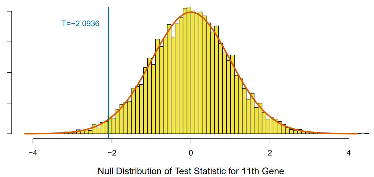
- Theoretical -value is . Re-sampling -value is
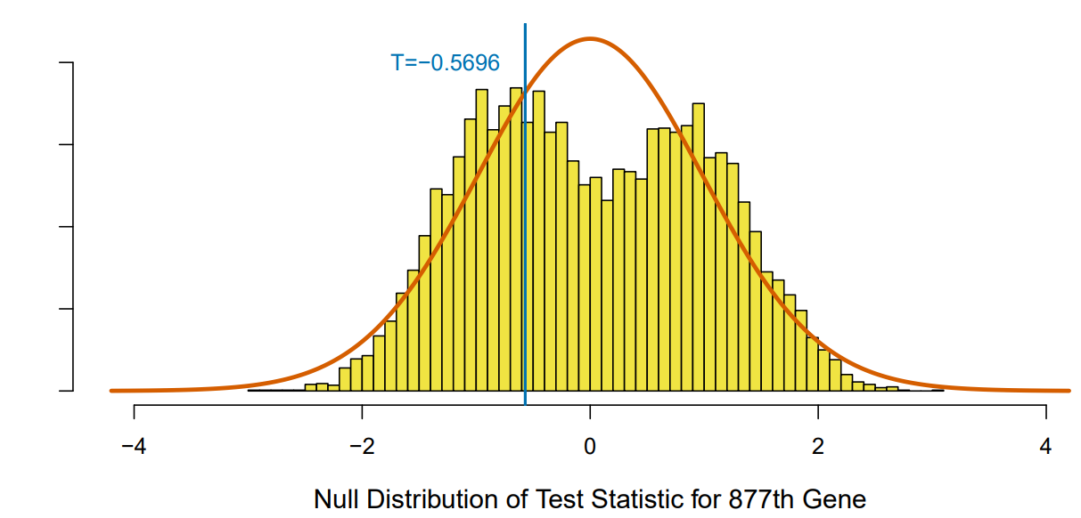
- Theoretical -value is . Re-sampling -value is
More on Re-Sampling Approaches
Re-samplingapproaches are useful if the theoreticalnull distributionis unavailable, or requires stringent assumptions- An extension of the re-sampling approach to compute a -value can be used to control
FDR - This example involved a two-sample -test, but similar approaches can be developed for other test statistics

AI, Security