Support Vector Machines

• Here we approach the two-class classification problem in a direct way :

  We try and find a plane that seperates the classes in feature space

• If we cannot, we get creative in two ways :
  • We soften what we mean by seperates, and
  • We enrich and enlarge the feature space so that separation is possible

What is a Hyperplane?

• A hyperplane in $p$ dimensions is a flat affine subspace of dimension $p-1$
• In general the equation for a hyperplane has the form
  $\beta_0+\beta_1X_1+\cdots+\beta_pX_p=0$
• In $p=2$ dimensions a hyperplane is a line
• If $\beta_0=0,$ the hyperplane goes throught the origin, otherwise not
• The vector $\beta=(\beta_1,\;\beta_2,\cdots,\beta_p)$ is called the normal vector - it points in a direction orthogonal to the surface of a hyperplane

Separating Hyperplanes

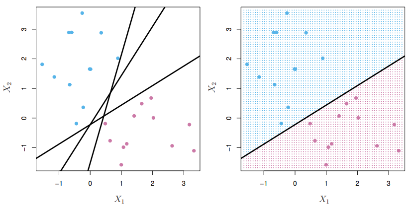
• If $f(X)=\beta_0+\beta_1X_1+\cdots+\beta_pX_p$, then $f(X)>0$ for points on one side of the hyperplane, and $f(X)<0$ for points on the other
• If we code the colored points as $Y_i=\pm1$ for blue, say, and $Y_i=-1$ for mauve, then if $Y_i\cdot f(X_i)>0$ for all $i$, $f(X)=0$ defines a separating hyperplane
  $d=\frac{|\beta_0+\beta_1X_1+\cdots+\beta_pX_p|}{\sqrt{\beta_1^2+\cdots+\beta_p^2}}$

Maximal Margin Classifier

• Among all seperating hyperplanes, find the one that makes the biggest gap or margin between the two classes
  
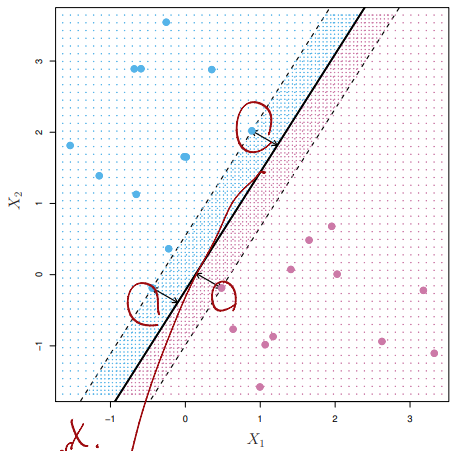
• Constrained optimization problem
  $\text{maximize M}\\[0.2cm] \text{subject to }\sum^p_{j=1}\beta^2_j=1\\[0.3cm] y_i(\beta_0+\beta_1x_{i1}+\cdots+\beta_px_{ip}\geq M,\quad\text{for all }i=1,\dots,N$

Non-separable Data

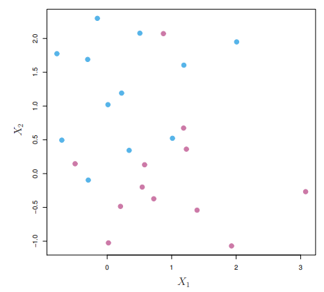
• The data are not separable by a linear boundary
• This is often the ase, unless $N<p$

Noisy Data

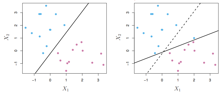
• Sometimes the data are separable, but noisy
• This can lead to a poor solution for the maximal-margin classifier
• The support vector classifier maximizes a soft margin

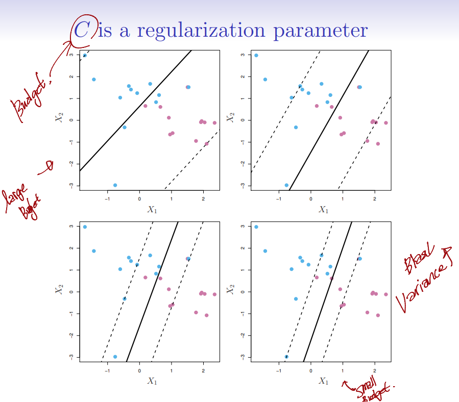
Support Vector Classifier

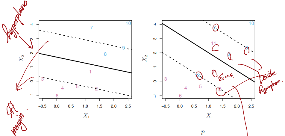
• $\epsilon_i$ : slack variable
• $C$ : Budget
  

Linear boundary can fail

• Sometimes a linear boundary simply won't work, no matter what value of $C$
• The example on the left is such a case. What to do?

Featue Expansion

• Enlarge the space of features by including transformations;
  e.g. $X^2_1,X^3_1,X_1X_2,X_1X^2_2,\dots$ Hence go from a $p$-dimensional space to a $M>p$ dimensional space
• Fit a support-vector classifier in the enlarged space
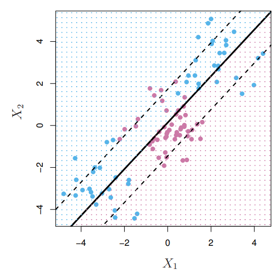
• This results in non-linear decision boundaries in the original space
• Example : Suppose we use $(X_1,X_2,X^2_1,X_2^2,X_1X_2)$ instead of just $(X_1,X_2)$. Then the decision boundary would be of the form
  $\beta_0+\beta_1X_1+\beta_2X_2+\beta_3X^2_1+\beta_4X^2_2+\beta_5X_1X_2=0$
• This leads to nonlinear decision boundaries in the original space(quadratic conic sections)

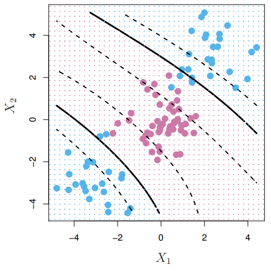
Cubic Polynomials

• Here we use a basis expansion of cubin polynomials
• From $2$ variables to $9$
• The support-vector classifier in the enlarged space solves the problem in the lower-dimensional space
  

Nonlinearities and Kernels

• Polynomials (especially high-dimensional ones) get wild rather fast
• There is a more elegant and controlled way to introduce nonlinearities in support-vector classifiers - through the use of kernels
• Before we discuss these, we must understand the role of inner products in support-vector classifiers

Inner products and Support Vectors

• The linear support vector classifier can be represented as
  $f(x)=\beta_0+\sum^n_{i=1}\alpha_i<x,x_i>\;:\text{n parameters}$
• To estimate the parameters $\alpha_1,\dots,\alpha_n$ and $\beta_0$, all we need are the $\left(\begin{matrix}n\\2\end{matrix}\right)$ inner products $<x_i,x_{i'}>$ between all pairs of training observations
• It turns out that most of the $\hat \alpha_i$ can be zero :
  $f(x)=\beta_0+\sum_{i\in S}\hat \alpha_i<x,x_i>$
• $S$ is the support set of indies $i$ such that $\hat \alpha_i >0$

Kernels and Support Vector Machines

• If we can compute inner-products between observations, we can fit a SV classifier. Can be quite abstract!
• Some special kernel functions can do this for us
  $K(x_i,x_{i'})=\left(1+\sum^p_{j=1}x_{ij}x_{i'j}\right)^d$
  computes this inner-products needed for $d$ dimensional polynomials - $\left(\begin{matrix}p+d\\d\end{matrix}\right)$ basis functions

  Try it for $p=2$ and $d=2$

• The solution has the form
  $f(x)=\beta_0+\sum_{i \in S}\hat \alpha_i K(x,x_i)$

Radial Kernel

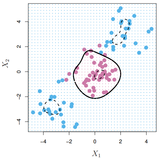
• Implict feature space; very high dimensional
• Controls variance by squashing down most dimensions severely

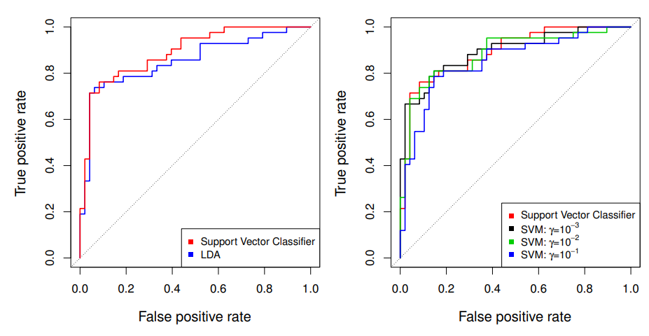
Example : Heart Data

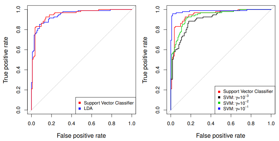
• ROC Curve is obtained by changing the threshold $0$ to threshold $t$ in $\hat f(X)>t$, and recording false positive and true positive rates as $t$ varies
• here we see ROC curves on training data
  

SVMs : more than 2 classes?

• The SVM as defined works for $K=2$ classes
• What do we do if we have $K>2$ classes?
  • OVA : One versus All.
    Fit $K$ different 2-class SVM classifiers $\hat f_k(x),\;k=1,\dots,K;$ each class versus the rest
    Classify $x^*$ to the class for which $\hat f_k(x^*)$
  • OVO : One versus One
    Fit all $\left(\begin{matrix}K\\2\end{matrix}\right)$ pairwise classifiers $\hat f_{kl}(x)$
    Classify $x^*$ to the class that wins the most pairwise competitions
• Which to choose? If $K$ is not too large, use OVO

Support Vector vs Logistic Regression?

• With $f(X)=\beta_0+\beta_1X_1+\cdots+\beta_pX_p$ can rephrase support-vector classifier optimization as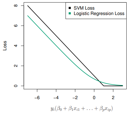

  $\min_{\beta_0,\dots,\beta_p}\left\{\sum^n_{i=1}\max\left[0,1-y_if(x_i)\right]+\lambda\sum^p_{j=1}\beta^2_j\right\}$

  

• This has the form loss plus penalty

• The loss is known as the hinge loss very similar to loss in logistic regression (negative log-likelihood)

Which to use : SVM or Logistic Regression

• When classes are (nearly) separable, SVM does better than LR. So does LDA
• When not, LR (with ridge penalty) and SVM very similar
• If you wish to estimate probabilities, LR is the choice
• For nonlinear boundaries, kernel SVMs are popular
• Can use kernels with LR and LDA as well, but computations are more expensive

All Contents written based on GIST - Machine Learning & Deep Learning Lesson(Instructor : Prof. sun-dong. Kim)