Image classification of flowers
Manually making image and label list
Image directories to dataset
Download & Extracting dataset folder in Google Cloud Storage While automatically (untar-True) the .tgz file
import os
from glob import glob
from PIL import Image

import numpy as np
import tensorflow as tf

import matplotlib.pyplot as plt

# 약 3,700장의 꽃 사진 데이터세트를 사용합니다.
# 아래 데이터 가져오기 그냥 사용합니다.

import pathlib
dataset_url = "https://storage.googleapis.com/download.tensorflow.org/example_images/flower_photos.tgz"
data_dir = tf.keras.utils.get_file('flower_photos', origin=dataset_url, untar=True)
data_dir = pathlib.Path(data_dir)
Downloading the dataset in a Current directory
import os
from glob import glob
from PIL import Image
import numpy as np
import matplotlib.pyplot as plt
import pathlib
import os
import pathlib
import tensorflow as tf

current_dir = os.getcwd()  # 현재 디렉터리 경로 가져오기
print(f"현재 디렉터리: {current_dir}")


dataset_url = "https://storage.googleapis.com/download.tensorflow.org/example_images/flower_photos.tgz"

current_dir = os.getcwd()  # 현재 디렉터리 경로 가져오기

try:
    data_dir = tf.keras.utils.get_file(
        'flower_photos',
        origin=dataset_url,
        untar=True,
        cache_dir=current_dir  # 현재 디렉터리 경로 지정
    )
    data_dir = pathlib.Path(data_dir)
    print(f"데이터 세트 다운로드 경로: {data_dir}")
except Exception as e:
    print(f"데이터 세트 다운로드 중 오류 발생: {e}")
The dataset is stored in TensorFlow’s cache directory (usually in ~/.keras/datasets/)
Converts the directory path into a Pathlib.Path object, making it easier to work with file paths. data_dir = pathlib.Path(data_dir)
Observe the folders inside the directory
!ls /root/.keras/datasets/flower_photos/flower_photos/

daisy  dandelion  LICENSE.txt  roses  sunflowers  tulips
Observe the number of .jpg file inside each folder
# daisy 폴더 안의 이지미 갯수
!ls -l /root/.keras/datasets/flower_photos/flower_photos/daisy | grep jpg | wc -l
633

# dandelion 폴더 안의 이지미 갯수
!ls -l /root/.keras/datasets/flower_photos/flower_photos/dandelion | grep jpg | wc -l
898

# roses 폴더 안의 이지미 갯수
!ls -l /root/.keras/datasets/flower_photos/flower_photos/roses | grep jpg | wc -l
641

# sunflowers 폴더 안의 이지미 갯수
!ls -l /root/.keras/datasets/flower_photos/flower_photos/sunflowers | grep jpg | wc -l
699

# tulips 폴더 안의 이지미 갯수
!ls -l /root/.keras/datasets/flower_photos/flower_photos/tulips | grep jpg | wc -l
799
using os.listdir and PIL.Image to read image files
# 이미지 패스 지정
daisy_path = '/root/.keras/datasets/flower_photos/flower_photos/daisy/'
dandelion_path = '/root/.keras/datasets/flower_photos/flower_photos/dandelion/'
roses_path = '/root/.keras/datasets/flower_photos/flower_photos/roses/'
sunflowers_path = '/root/.keras/datasets/flower_photos/flower_photos/sunflowers/'
tulips_path = '/root/.keras/datasets/flower_photos/flower_photos/tulips/'

# 이미지 패스의 파말 리스트 만들기
daisy_file = os.listdir(daisy_path)
dandelion_file = os.listdir(dandelion_path)
roses_file = os.listdir(roses_path)
sunflowers_file = os.listdir(sunflowers_path)
tulips_file = os.listdir(tulips_path)
Making dataset list Manually
# Class 라벨 정의

class2idx = {'daisy' :  0, 'dandelion' : 1,  'roses' : 2, 'sunflowers' : 3, 'tulips' : 4}
idx2class = {0 : 'daisy', 1 : 'dandelion', 2 : 'roses', 3 : 'sunflowers', 4 : 'tulips'}

# 수작업으로 이미지 리스트와 라벨 리스트 만들기

img_list = []
label_list = []

daisy_file = os.listdir(daisy_path)
for img_file in daisy_file :
  img = Image.open(daisy_path + img_file).resize((128,128))
  img = np.array(img)/255.  # 이미지 스케일링
  img_list.append(img)
  label_list.append(0) # daisy : 0

dandelion_file = os.listdir(dandelion_path)
for img_file in dandelion_file :
  img = Image.open(dandelion_path + img_file).resize((128,128))
  img = np.array(img)/255.  # 이미지 스케일링
  img_list.append(img)
  label_list.append(1) # dandelion : 1

roses_file = os.listdir(roses_path)
for img_file in roses_file :
  img = Image.open(roses_path + img_file).resize((128,128))
  img = np.array(img)/255.  # 이미지 스케일링
  img_list.append(img)
  label_list.append(2) # roses : 2

sunflowers_file = os.listdir(sunflowers_path)
for img_file in sunflowers_file :
  img = Image.open(sunflowers_path + img_file).resize((128,128))
  img = np.array(img)/255.  # 이미지 스케일링
  img_list.append(img)
  label_list.append(3) # sunflowers : 2

tulips_file = os.listdir(tulips_path)
for img_file in tulips_file :
  img = Image.open(tulips_path + img_file).resize((128,128))
  img = np.array(img)/255.  # 이미지 스케일링
  img_list.append(img)
  label_list.append(4) # tulips : 2


# Numpy for tensorflow operation
 # 이미지 리스트, 라벨 리스트루 numpy array 변경
img_list_arr = np.array(img_list)
label_list_arr = np.array(label_list)

from sklearn.model_selection import train_test_split

X_train, X_test , y_train, y_test = train_test_split(img_list_arr, label_list_arr, test_size=0.3, stratify=label_list_arr, random_state=41)
X_train.shape, X_test.shape , y_train.shape, y_test.shape
((2569, 128, 128, 3), (1101, 128, 128, 3), (2569,), (1101,))
Building CNN model for classfication
# Hyperparameter Tunning

num_epochs = 10
batch_size = 32

learning_rate = 0.001
dropout_rate = 0.5

input_shape = (128, 128, 3)  # 사이즈 확인

# Sequential 모델 정의
from tensorflow.keras.models import Sequential
from tensorflow.keras.layers import Dense, Dropout, Flatten, Conv2D, MaxPooling2D

model = Sequential()
model.add(Conv2D(32, kernel_size=(5,5), strides=(1,1), padding='same', activation='relu', input_shape=input_shape))
model.add(MaxPooling2D(pool_size=(2,2), strides=(2,2)))
model.add(Conv2D(64,(2,2), activation='relu', padding='same'))
model.add(MaxPooling2D(pool_size=(2,2)))
model.add(Dropout(0.2))
model.add(Flatten())
model.add(Dense(128, activation='relu'))
model.add(Dropout(0.3))
model.add(Dense(5, activation='softmax'))

# 모델 컴파일
model.compile(optimizer=tf.keras.optimizers.Adam(learning_rate),  # Optimization
              loss='sparse_categorical_crossentropy',  # Loss Function
              metrics=['accuracy'])  # Metrics / Accuracy


model.summary()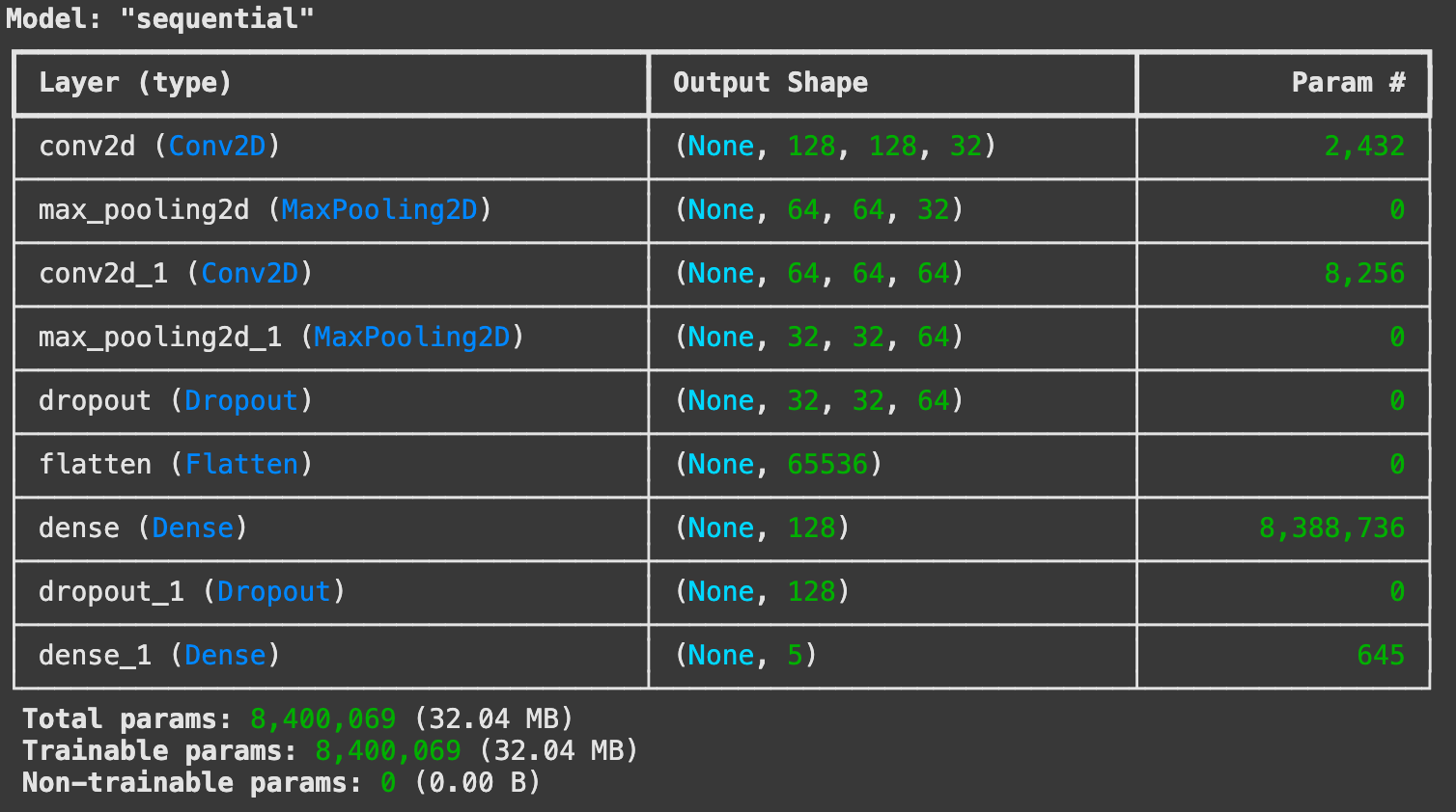
# callback : EarlyStopping, ModelCheckpoint

from tensorflow.keras.callbacks import EarlyStopping, ModelCheckpoint

# EarlyStopping
es = EarlyStopping(monitor='val_loss', mode='min', verbose=1, patience=5)

# ModelCheckpoint
checkpoint_path = "my_checkpoint.keras"
checkpoint = ModelCheckpoint(filepath=checkpoint_path,
                             save_best_only=True,
                             monitor='val_loss',
                             verbose=1)
num_epochs = 10
batch_size = 32

# 모델 학습(fit)
history = model.fit(
    X_train, y_train ,
    validation_data=(X_test, y_test),
    epochs=num_epochs,
    batch_size=batch_size,
    callbacks=[es, checkpoint]
)

Epoch 1/10
81/81 ━━━━━━━━━━━━━━━━━━━━ 0s 848ms/step - accuracy: 0.3299 - loss: 1.8679
Epoch 1: val_loss improved from inf to 1.17802, saving model to my_checkpoint.keras
81/81 ━━━━━━━━━━━━━━━━━━━━ 83s 989ms/step - accuracy: 0.3308 - loss: 1.8629 - val_accuracy: 0.5095 - val_loss: 1.1780
Epoch 2/10
81/81 ━━━━━━━━━━━━━━━━━━━━ 0s 847ms/step - accuracy: 0.5675 - loss: 1.0859
Epoch 2: val_loss improved from 1.17802 to 1.06809, saving model to my_checkpoint.keras
81/81 ━━━━━━━━━━━━━━━━━━━━ 81s 982ms/step - accuracy: 0.5676 - loss: 1.0858 - val_accuracy: 0.5840 - val_loss: 1.0681
Epoch 3/10
81/81 ━━━━━━━━━━━━━━━━━━━━ 0s 842ms/step - accuracy: 0.6651 - loss: 0.9232
Epoch 3: val_loss did not improve from 1.06809
81/81 ━━━━━━━━━━━━━━━━━━━━ 78s 970ms/step - accuracy: 0.6651 - loss: 0.9230 - val_accuracy: 0.5658 - val_loss: 1.1227
Epoch 4/10
81/81 ━━━━━━━━━━━━━━━━━━━━ 0s 822ms/step - accuracy: 0.6777 - loss: 0.8071
Epoch 4: val_loss improved from 1.06809 to 1.03832, saving model to my_checkpoint.keras
81/81 ━━━━━━━━━━━━━━━━━━━━ 81s 959ms/step - accuracy: 0.6783 - loss: 0.8060 - val_accuracy: 0.6240 - val_loss: 1.0383
Epoch 5/10
81/81 ━━━━━━━━━━━━━━━━━━━━ 0s 812ms/step - accuracy: 0.8141 - loss: 0.5233
Epoch 5: val_loss did not improve from 1.03832
81/81 ━━━━━━━━━━━━━━━━━━━━ 73s 899ms/step - accuracy: 0.8142 - loss: 0.5232 - val_accuracy: 0.6104 - val_loss: 1.1100
Epoch 6/10
81/81 ━━━━━━━━━━━━━━━━━━━━ 0s 846ms/step - accuracy: 0.8927 - loss: 0.3319
Epoch 6: val_loss did not improve from 1.03832
81/81 ━━━━━━━━━━━━━━━━━━━━ 76s 944ms/step - accuracy: 0.8926 - loss: 0.3321 - val_accuracy: 0.6140 - val_loss: 1.1934
Epoch 7/10
81/81 ━━━━━━━━━━━━━━━━━━━━ 0s 835ms/step - accuracy: 0.9318 - loss: 0.2382
Epoch 7: val_loss did not improve from 1.03832
81/81 ━━━━━━━━━━━━━━━━━━━━ 84s 963ms/step - accuracy: 0.9317 - loss: 0.2383 - val_accuracy: 0.5931 - val_loss: 1.3962
Epoch 8/10
81/81 ━━━━━━━━━━━━━━━━━━━━ 0s 912ms/step - accuracy: 0.9503 - loss: 0.1794
Epoch 8: val_loss did not improve from 1.03832
81/81 ━━━━━━━━━━━━━━━━━━━━ 85s 1s/step - accuracy: 0.9503 - loss: 0.1794 - val_accuracy: 0.5995 - val_loss: 1.5562
Epoch 9/10
81/81 ━━━━━━━━━━━━━━━━━━━━ 0s 850ms/step - accuracy: 0.9581 - loss: 0.1308
Epoch 9: val_loss did not improve from 1.03832
81/81 ━━━━━━━━━━━━━━━━━━━━ 79s 968ms/step - accuracy: 0.9581 - loss: 0.1308 - val_accuracy: 0.6058 - val_loss: 1.5337
Epoch 9: early stopping
Performance graph
history.history.keys()
dict_keys(['accuracy', 'loss', 'val_accuracy', 'val_loss'])

plt.plot(history.history['accuracy'], label='Accuracy')
plt.plot(history.history['val_accuracy'], label='Val Accuracy')
plt.xlabel('Epoch')
plt.ylabel('Accuracy')
plt.legend()
plt.title('Model Accuracy')
plt.show()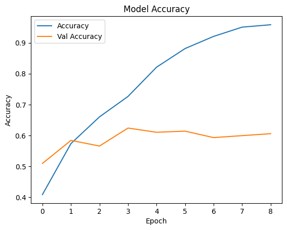
# Test 데이터로 성능 예측하기

i=1
plt.figure(figsize=(16, 8))
for img, label in zip(X_test[:8], y_test[:8]):
      # 모델 예측(predict)
      pred = model.predict(img.reshape(-1,128, 128, 3))
      pred_t = np.argmax(pred)
      plt.subplot(2, 4, i)
      plt.title(f'True Value:{label}, Pred Value: {pred_t}')
      plt.imshow(img)
      plt.axis('off')
      i = i + 1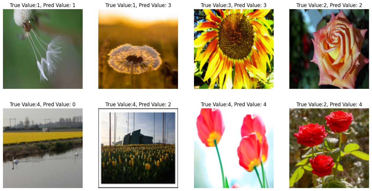
Making dataset using function - image_dataset_from_directory
Download & Extracting dataset folder in Google Cloud Storage While automatically (untar-True) the .tgz file
import os
from glob import glob
from PIL import Image

import numpy as np
import tensorflow as tf

import matplotlib.pyplot as plt

# 약 3,700장의 꽃 사진 데이터세트를 사용합니다.
# 아래 데이터 가져오기 그냥 사용합니다.

import pathlib
dataset_url = "https://storage.googleapis.com/download.tensorflow.org/example_images/flower_photos.tgz"
data_dir = tf.keras.utils.get_file('flower_photos', origin=dataset_url, untar=True)
data_dir = pathlib.Path(data_dir)
The dataset is stored in TensorFlow’s cache directory (usually in ~/.keras/datasets/)
Converts the directory path into a Pathlib.Path object, making it easier to work with file paths. data_dir = pathlib.Path(data_dir)
Observe the folders inside the directory
!ls /root/.keras/datasets/flower_photos/flower_photos/

daisy  dandelion  LICENSE.txt  roses  sunflowers  tulips
Observe the number of .jpg file inside each folder
# daisy 폴더 안의 이지미 갯수
!ls -l /root/.keras/datasets/flower_photos/flower_photos/daisy | grep jpg | wc -l
633

# dandelion 폴더 안의 이지미 갯수
!ls -l /root/.keras/datasets/flower_photos/flower_photos/dandelion | grep jpg | wc -l
898

# roses 폴더 안의 이지미 갯수
!ls -l /root/.keras/datasets/flower_photos/flower_photos/roses | grep jpg | wc -l
641

# sunflowers 폴더 안의 이지미 갯수
!ls -l /root/.keras/datasets/flower_photos/flower_photos/sunflowers | grep jpg | wc -l
699

# tulips 폴더 안의 이지미 갯수
!ls -l /root/.keras/datasets/flower_photos/flower_photos/tulips | grep jpg | wc -l
799
Automatically generating dataset and labeling using image_dataset_from_directory
# 하이터 파라미터 정의
input_shape = (224, 224, 3)
batch_size = 32
num_classes = 5

# 이미지 패스 지정
img_path ='/root/.keras/datasets/flower_photos/flower_photos/'

# image_dataset_from_directory 함수 활용하여
# 이미지 폴더 밑의 이미지들에 대해 원핫인코딩된 labeling수행, 이미지 배치, 셔플 수행

# Train Dataset 만들기
train_ds = tf.keras.preprocessing.image_dataset_from_directory(
                                             directory=img_path,
                                             label_mode="categorical",   # binary , categorical
                                             batch_size=batch_size,
                                             image_size=(224, 224),      # 사이즈 확인
                                             seed=42,
                                             shuffle=True,
                                             validation_split=0.2,
                                             subset="training"    # One of "training" or "validation". Only used if validation_split is set.
                                            )

# Test Dataset 만들기
test_ds = tf.keras.preprocessing.image_dataset_from_directory(
                                             directory=img_path,
                                             label_mode="categorical",   # binary , categorical
                                             batch_size=batch_size,
                                             image_size=(224, 224),      # 사이즈 확인
                                             seed=42,
                                             validation_split=0.2,
                                             subset="validation"    # One of "training" or "validation". Only used if validation_split is set.
                                            )

Found 3670 files belonging to 5 classes.
Using 2936 files for training.
Found 3670 files belonging to 5 classes.
Using 734 files for validation.
Check the made dataset
# Class 이름 확인
train_ds.class_names
['daisy', 'dandelion', 'roses', 'sunflowers', 'tulips']

# 40,000건 중에서 32,000건 Train 사용. test용으로 8,000건 사용
len(train_ds) * 32 , len(test_ds) * 32
(2944, 736)

batch_img, batch_label = next(iter(train_ds))
batch_img.shape, batch_label.shape
(TensorShape([32, 224, 224, 3]), TensorShape([32, 5]))
Build model
# Hyperparameter Tunning

num_epochs = 10
batch_size = 32

learning_rate = 0.001
dropout_rate = 0.5

input_shape = (224, 224, 3)  # 사이즈 확인
num_classes = 5

from tensorflow.keras.models import Sequential
from tensorflow.keras.layers import Dense, Dropout, Flatten, Conv2D, MaxPooling2D, Rescaling, Input

from tensorflow.keras.models import Model

# model = Sequential()
# model.add(Rescaling(1. / 255))  # 이미지 Rescaling. 없이 하면 성능이 안나옴.
# model.add(Conv2D(32, kernel_size=(5,5), strides=(1,1), padding='same', activation='relu', input_shape=input_shape))
# model.add(MaxPooling2D(pool_size=(2,2), strides=(2,2)))
# model.add(Conv2D(64,(2,2), activation='relu', padding='same'))
# model.add(MaxPooling2D(pool_size=(2,2)))
# model.add(Dropout(0.2))
# model.add(Flatten())
# model.add(Dense(128, activation='relu'))
# model.add(Dropout(0.3))
# model.add(Dense(5, activation='softmax'))

# 입력 이미지 크기 정의
input_shape = (224, 224, 3)

# Functional API를 사용한 모델 구성
inputs = Input(shape=input_shape)  # Input 레이어 명시적으로 정의
x = Rescaling(1./255)(inputs) # Rescaling을 Input 다음에 위치시킴
x = Conv2D(32, kernel_size=(5, 5), strides=(1, 1), padding='same', activation='relu')(x)
x = MaxPooling2D(pool_size=(2, 2), strides=(2, 2))(x)
x = Conv2D(64, (2, 2), activation='relu', padding='same')(x)
x = MaxPooling2D(pool_size=(2, 2))(x)
x = Dropout(0.2)(x)
x = Flatten()(x)
x = Dense(128, activation='relu')(x)
x = Dropout(0.3)(x)
x = Dense(5, activation='softmax')(x)  # 출력 레이어, 5개의 클래스

model = Model(inputs=inputs, outputs=x)

model.summary()

# Model compile
model.compile(optimizer=tf.keras.optimizers.Adam(learning_rate),  # Optimization
              loss='categorical_crossentropy',  # Loss Function
              metrics=['accuracy'])  # Metrics / Accuracy

from tensorflow.keras.callbacks import EarlyStopping, ModelCheckpoint

# EarlyStopping
es = EarlyStopping(monitor='val_loss', mode='min', verbose=1, patience=3)

# ModelCheckpoint
checkpoint_path = "my_checkpoint.keras"
checkpoint = ModelCheckpoint(filepath=checkpoint_path,
                             save_best_only=True,
                             monitor='val_loss',
                             verbose=1)

# image_dataset_from_directory 이용하여 데이터 만들었을때 아래와 같이 학습 진행
# num_epochs = 10

# 모델 학습(fit)
history = model.fit(
    train_ds,
    validation_data=(test_ds),
    epochs=10,
    callbacks=[es, checkpoint]
)

Epoch 1/10
92/92 ━━━━━━━━━━━━━━━━━━━━ 0s 3s/step - accuracy: 0.2657 - loss: 4.5210
Epoch 1: val_loss improved from inf to 1.25579, saving model to my_checkpoint.keras
92/92 ━━━━━━━━━━━━━━━━━━━━ 277s 3s/step - accuracy: 0.2664 - loss: 4.4974 - val_accuracy: 0.5204 - val_loss: 1.2558
Epoch 2/10
92/92 ━━━━━━━━━━━━━━━━━━━━ 0s 3s/step - accuracy: 0.4396 - loss: 1.2907
Epoch 2: val_loss improved from 1.25579 to 1.16467, saving model to my_checkpoint.keras
92/92 ━━━━━━━━━━━━━━━━━━━━ 266s 3s/step - accuracy: 0.4399 - loss: 1.2905 - val_accuracy: 0.5368 - val_loss: 1.1647
Epoch 3/10
92/92 ━━━━━━━━━━━━━━━━━━━━ 0s 3s/step - accuracy: 0.5151 - loss: 1.1689
Epoch 3: val_loss improved from 1.16467 to 1.06240, saving model to my_checkpoint.keras
92/92 ━━━━━━━━━━━━━━━━━━━━ 274s 3s/step - accuracy: 0.5154 - loss: 1.1686 - val_accuracy: 0.5436 - val_loss: 1.0624
Epoch 4/10
92/92 ━━━━━━━━━━━━━━━━━━━━ 0s 3s/step - accuracy: 0.5998 - loss: 1.0108
Epoch 4: val_loss improved from 1.06240 to 1.00894, saving model to my_checkpoint.keras
92/92 ━━━━━━━━━━━━━━━━━━━━ 275s 3s/step - accuracy: 0.6000 - loss: 1.0105 - val_accuracy: 0.6144 - val_loss: 1.0089
Epoch 5/10
92/92 ━━━━━━━━━━━━━━━━━━━━ 0s 3s/step - accuracy: 0.6680 - loss: 0.8557
Epoch 5: val_loss did not improve from 1.00894
92/92 ━━━━━━━━━━━━━━━━━━━━ 269s 3s/step - accuracy: 0.6681 - loss: 0.8555 - val_accuracy: 0.6117 - val_loss: 1.0112
Epoch 6/10
92/92 ━━━━━━━━━━━━━━━━━━━━ 0s 3s/step - accuracy: 0.7233 - loss: 0.7225
Epoch 6: val_loss did not improve from 1.00894
92/92 ━━━━━━━━━━━━━━━━━━━━ 267s 3s/step - accuracy: 0.7234 - loss: 0.7221 - val_accuracy: 0.5981 - val_loss: 1.1158
Epoch 7/10
92/92 ━━━━━━━━━━━━━━━━━━━━ 0s 3s/step - accuracy: 0.7865 - loss: 0.5713
Epoch 7: val_loss did not improve from 1.00894
92/92 ━━━━━━━━━━━━━━━━━━━━ 272s 3s/step - accuracy: 0.7867 - loss: 0.5711 - val_accuracy: 0.5763 - val_loss: 1.2445
Epoch 7: early stopping
Prediction and graph
history.history.keys()

dict_keys(['accuracy', 'loss', 'val_accuracy', 'val_loss'])

plt.plot(history.history['accuracy'], label='Accuracy')
plt.plot(history.history['val_accuracy'], label='Val Accuracy')
plt.xlabel('Epoch')
plt.ylabel('Accuracy')
plt.legend()
plt.title('Model Accuracy')
plt.show()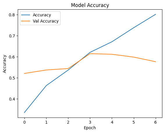
len(test_ds) * 32
736

# 배치사이즈 이미지/라벨 가져오기
batch_img , batch_label = next(iter(test_ds))
type(batch_img), batch_img.shape
(tensorflow.python.framework.ops.EagerTensor, TensorShape([32, 224, 224, 3]))

# Test 데이터로 성능 예측하기

i = 1
plt.figure(figsize=(16, 30))
for img, label in list(zip(batch_img, batch_label)):
    pred = model.predict(img.numpy().reshape(-1, 224,224,3), verbose=0)
    pred_t = np.argmax(pred)
    plt.subplot(8, 4, i)
    plt.title(f'True Value:{np.argmax(label)}, Pred Value: {pred_t}')
    plt.imshow(img/255)  # 이미지 픽셀값들이 실수형이므로 0~1 사이로 변경해야 에러 안남
    i = i + 1
Fine Tuning MobileNetV3
obtaining base model from tf.keras.applications
# 케라스 applicatioins에 어떤 종류의 모델 있는지 확인
dir(tf.keras.applications)

# 사전 훈련된 모델 MobileNetV2에서 기본 모델을 생성합니다.
# 아래와 같은 형식을 MobileNetV2 Transfer Learning 사용하며 됩니다.

base_model = tf.keras.applications.MobileNetV2(input_shape=(224, 224, 3), weights='imagenet', include_top=False)
dir(tf.keras.applications)
🔹 This lists all pre-trained models available in Keras Applications.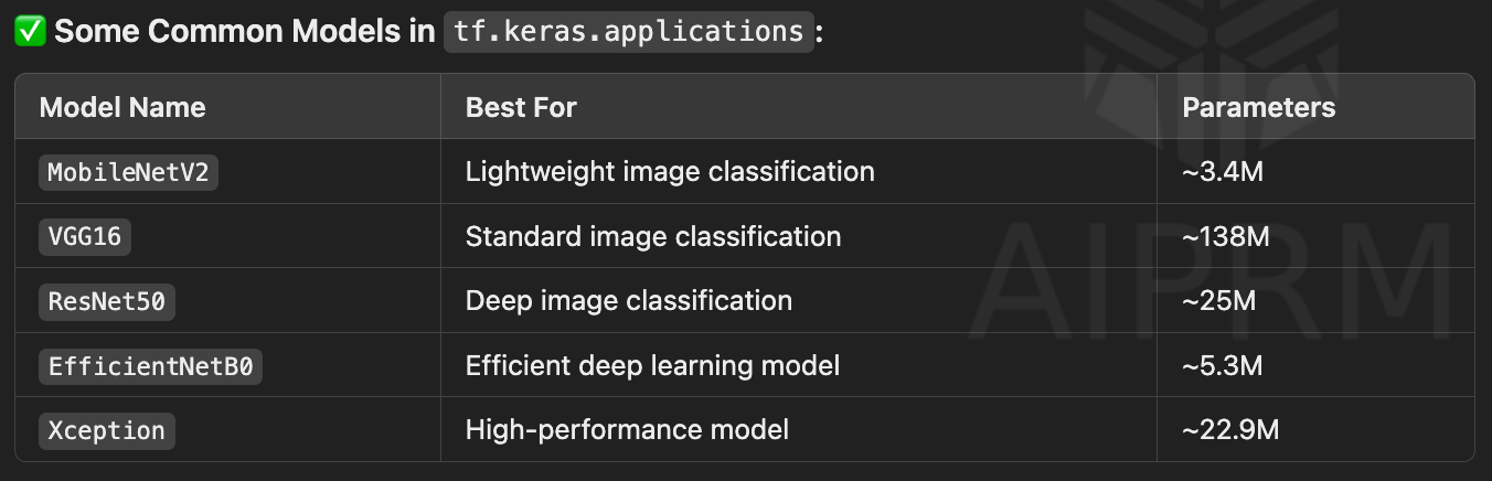
🔹 Breakdown of Parameters
input_shape=(224, 224, 3)
The model expects input images of size 224x224 pixels with 3 channels (RGB).
If images are a different size, they must be resized before feeding them into the model.
weights='imagenet'
Loads pre-trained weights from the ImageNet dataset.
The model has already learned useful features from millions of images.
include_top=False
Excludes the fully connected (FC) layer at the top of the model.
This means the model will only output feature maps, which can be used for Transfer Learning.
*Full list of Parameters for loading pretrained model
this code might include classifier layers but it ""should not"" for the following code
tf.keras.applications.MobileNetV2(
    input_shape=(224, 224, 3),   # Image size (height, width, channels)
    alpha=1.0,                   # Width multiplier (model size adjustment)
    include_top=True,            # Whether to include the classification layer
    weights="imagenet",          # Pre-trained weights (or None for random initialization)
    input_tensor=None,           # Custom input tensor
    pooling=None,                # Pooling type: None, 'avg', 'max'
    classes=1000,                # Number of output classes
    classifier_activation="softmax"  # Activation function for classification
)
linear probing the model (should not include the code above)
preprocessing input value from [0, 255] -> [-1, 1]
# tf.keras.applications.MobileNetV2 모델은 [-1, 1]의 픽셀 값을 예상하지만 이 시점에서 이미지의 픽셀 값은 [0, 255]입니다.
# MobileNetV2 모델에서 제대로 수행하기 위해 크기를 [-1, 1]로 재조정해야 합니다.(안하고 수행해도 성능 잘 나옴)
# 방법 2가지 있음
# 첫번째 방법 : preprocess_input = tf.keras.applications.mobilenet_v2.preprocess_input
# 두번째 방법 : rescale = tf.keras.layers.Rescaling(1./127.5, offset=-1)
preprocess_input = tf.keras.applications.mobilenet_v2.preprocess_input
making the pretrained model freezed
# MobileNet V2 베이스 모델 고정하기
base_model.trainable = False
adding classifier layers
# 모델 구축 : 이미지 픽셀값 조정 수행하기(Rescaling) --> 성능 더 잘 나옴.

inputs = tf.keras.Input(shape=(224, 224, 3))
x = tf.keras.layers.Rescaling(1./127.5, offset=-1)(inputs)
x = base_model(x, training=False)
x = tf.keras.layers.GlobalAveragePooling2D()(x)  # 3차원(7, 7, 1280) --> 1차원(1280)으로 줄이기 : GlobalAveragePooling2D
output = tf.keras.layers.Dense(5, activation='softmax')(x)

model = tf.keras.Model(inputs=inputs, outputs=output)
model.summary()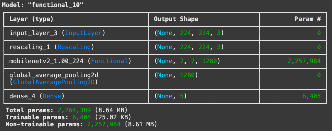
training the model
# 모델 compile

model.compile(optimizer=tf.keras.optimizers.Adam(learning_rate),  # Optimization
              loss='categorical_crossentropy',  # Loss Function
              metrics=['accuracy'])             # Metrics / Accuracy

from tensorflow.keras.callbacks import EarlyStopping, ModelCheckpoint

# EarlyStopping
es = EarlyStopping(monitor='val_loss', mode='min', verbose=1, patience=3)

# ModelCheckpoint
checkpoint_path = "my_checkpoint.keras"
checkpoint = ModelCheckpoint(filepath=checkpoint_path,
                             save_best_only=True,
                             monitor='val_loss',
                             verbose=1)

# image_dataset_from_directory 이용하여 DataSet을 만들었으며
# num_epochs = 10
# batch_size = 32

history = model.fit(
    train_ds,
    validation_data = test_ds,
    epochs=2,
    callbacks=[es, checkpoint]
)
Epoch 1/2
92/92 ━━━━━━━━━━━━━━━━━━━━ 0s 1s/step - accuracy: 0.6204 - loss: 1.0105
Epoch 1: val_loss improved from inf to 0.43213, saving model to my_checkpoint.keras
92/92 ━━━━━━━━━━━━━━━━━━━━ 159s 2s/step - accuracy: 0.6218 - loss: 1.0072 - val_accuracy: 0.8638 - val_loss: 0.4321
Epoch 2/2
92/92 ━━━━━━━━━━━━━━━━━━━━ 0s 1s/step - accuracy: 0.8664 - loss: 0.3784
Epoch 2: val_loss improved from 0.43213 to 0.37288, saving model to my_checkpoint.keras
92/92 ━━━━━━━━━━━━━━━━━━━━ 196s 2s/step - accuracy: 0.8665 - loss: 0.3781 - val_accuracy: 0.8706 - val_loss: 0.3729history.history.keys()
dict_keys(['accuracy', 'loss', 'val_accuracy', 'val_loss'])
plt.plot(history.history['accuracy'], label='Accuracy')
plt.plot(history.history['val_accuracy'], label='Val Accuracy')
plt.xlabel('Epoch')
plt.ylabel('Accuracy')
plt.legend()
plt.title('Model Accuracy')
plt.show()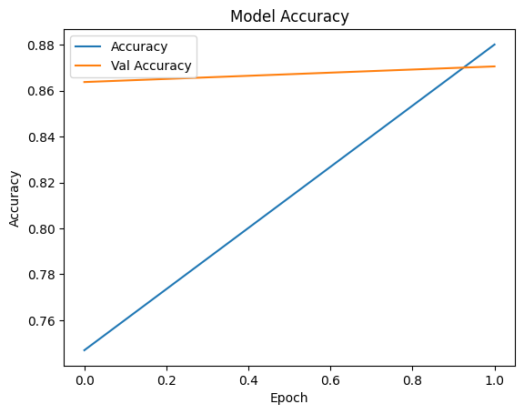
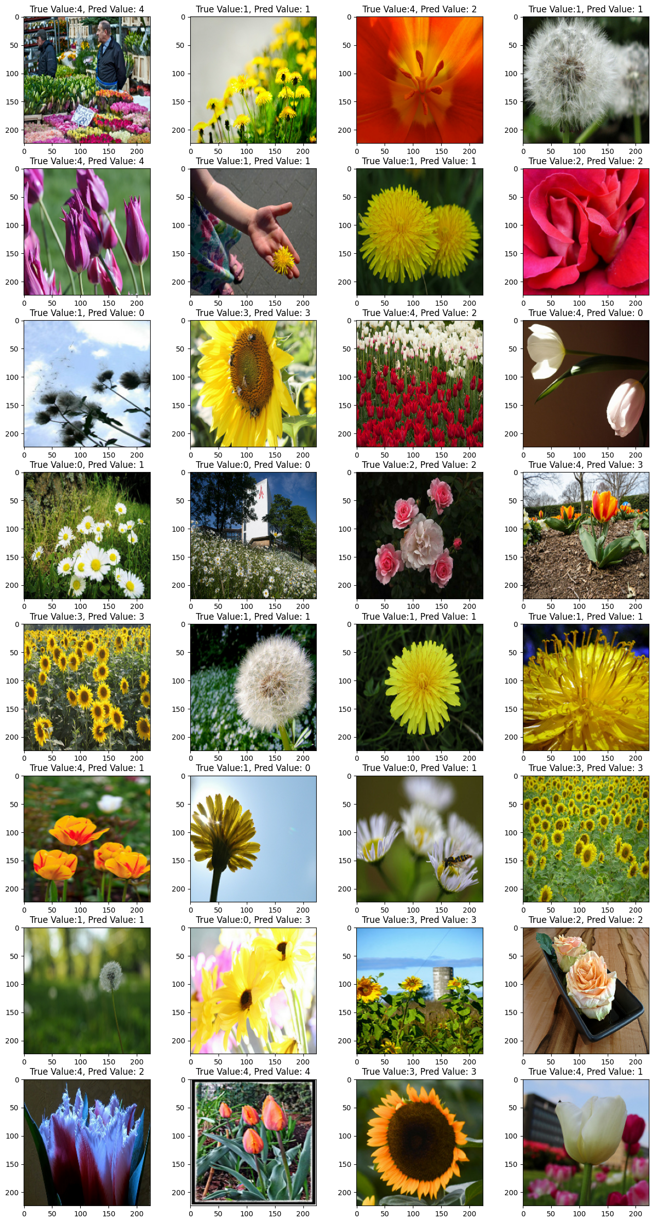
Observe prediction
# test_generator 샘플 데이터 가져오기
# 배치 사이즈 32 확인

batch_img, batch_label = next(iter(test_ds))
print(batch_img.shape)
print(batch_label.shape)
(32, 224, 224, 3)
(32, 5)

# 이미지 rescale 되어 있는 상태
batch_img[0][0][:10]
<tf.Tensor: shape=(10, 3), dtype=float32, numpy=
array([[ 69.68112  ,  60.482143 ,  19.229591 ],
       [ 19.790815 ,  24.058674 ,  20.165815 ],
       [  6.683674 ,   9.448984 ,   4.8316326],
       [  9.142857 ,  19.160713 ,   6.839285 ],
       [ 41.05103  ,  34.045925 ,  16.109695 ],
       [ 16.948978 ,  16.846937 ,  17.020407 ],
       [ 48.051018 ,  58.512745 ,  41.510197 ],
       [ 84.142845 , 108.362236 ,  87.528046 ],
       [ 27.025509 ,  28.267847 ,  20.464289 ],
       [ 33.33163  ,  44.859703 ,  31.765312 ]], dtype=float32)>

# 100% 성능 보여줌

i = 1
plt.figure(figsize=(16, 30))
for img, label in list(zip(batch_img, batch_label)):
    pred = model.predict(img.numpy().reshape(-1, 224,224,3), verbose=0)
    pred_t = np.argmax(pred)
    plt.subplot(8, 4, i)
    plt.title(f'True Value:{np.argmax(label)}, Pred Value: {pred_t}')
    plt.imshow(img/255)  # 이미지 픽셀값들이 실수형이므로 0~1 사이로 변경해야 에러 안남
    i = i + 1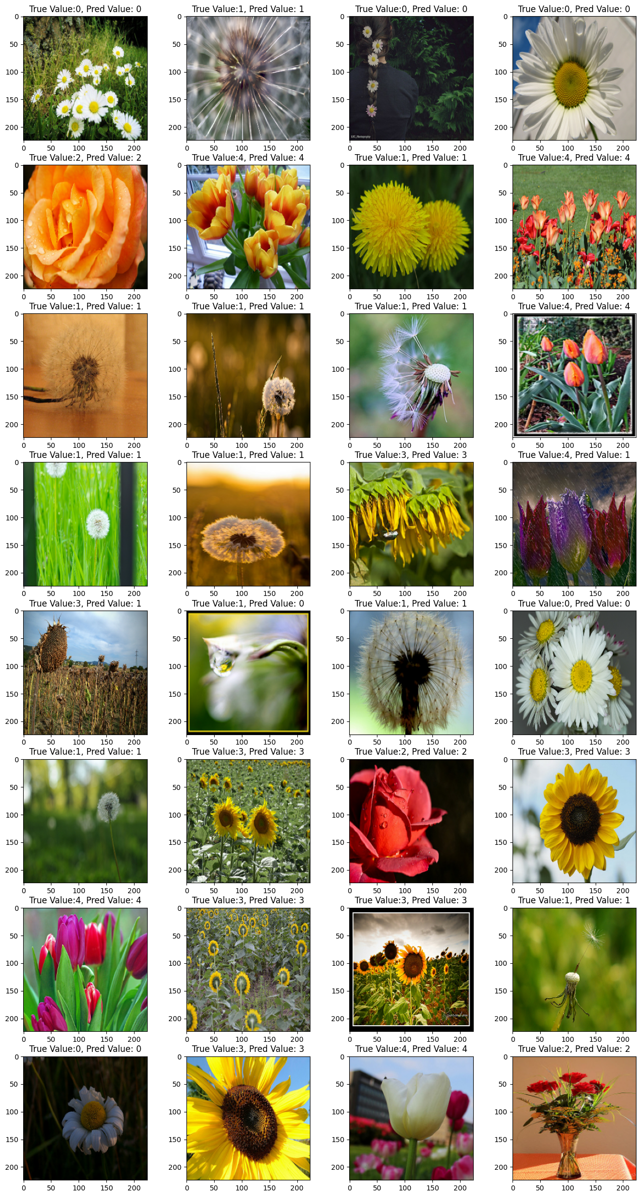

AI, Graphics, Medical Imaging