Informer: Beyond Efficient Transformer for Long Sequence Time-Series Forecasting

22년 11월에 읽었던 논문을 거의 1년이 지나가서야 블로그에 업로드 하게 됐다. 이미 word로 정리는 해뒀지만 때를 놓쳤다가 복습할겸해서 업로드를 한다.
이 논문 말고도 쌓여있는 논문이 너무 많다.

Abstract

Long Sequence Time-Series Forecasting(LSTF)는 모델의 높은 예측능력을 요구한다. 과거와 현재를 효과적으로 Coupling 하는 능력을 요구하고 최근의 연구인 Transformer는 이 측면에 대해서 잠재력을 보여줬다
하지만 바로 LSTF에 적용하기에는 몇가지 Transformer에 관한 문제들이 있는데
1. Quadratic 한 Time Complexity
2. High memory usage
3. encoder-decoder architecture 내재된 한계

모델은 3가지의 특성을 지니고 있는데

1.Self-attention에서 ProbSparse를 사용해서 time complexity O(L log L)와 memory usage를 낮췄음에도 Transformer와 비교했을때 sequence의 dependency 부분에서 비슷한 성능을 냈다.

2.Self-attention에서 dominating한 attention을 강조했다.

3.Generative style decoder 로써 long time-series sequence를 한번의 forward operation을 통해 예측한다

Introduction

Time-series forecasting은 여러 domain에 걸쳐 critical한 요소이다.
우리는 많은 양의 과거에 대한 Time series Data를 LSTF(Long Sequence Timeseries Forecasting)를 위해 사용할 수 있다.
하지만, 현존하는 방법론들은 대부분 short-term 문제를 풀기 위해 고안된 것이 많다. Short-term예측이라고 하면 48개 이하의 시점에 대한 예측을 말한다

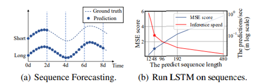
(a), Figure는 LSTF가 short sequence prediction보다 더 많은 period를 커버할 수 있음을 보여주고
(b), Figure는 현존하는 모델들이 LSTF에 대한 Performance가 떨어짐을 보여준다

->초당 예측길이가 sequence length가 길어지면 길어질수록 계속해서 떨어지고 있고, MSE Score또한 지속적으로 올라감을 볼 수 있다

LSTF에대한 Major Challenge는 Long Sequence에 대한 수요를 충족시키기 위해 예측능력을 강화 하는 것에 있다. 다음과 같은 것을 요구하는데
(a) 뛰어난 long-range alignment ability
(=과거 데이터를 얼마나 반영할 수 있느냐)
(b) Long sequence input과 output에 대한 효율적인 계산

• 최근에 Transformer 모델은 Long-range dependency capturing 하는 것에 대해서 매우 뛰어난 Performance를 보여줬다
• Transformer의 self-attention mechanism은 Recurrent한 구조를 사용하지 않기 때문에 maximum path length가 O(1)[Theoretical Shortest]이 된다
  
  Maximum path length: 특정 시점의 Token을 과거 시점의 Token과 비교하고 싶을 때 필요한 계산 횟수이다 RNN의 경우 특정 token이 매 RNN cell에서 들어가기 때문에 a시점에서의 토큰과 과거 시점 b사이의 토큰을 비교하고 싶으면 a-b만큼의 연산이 필요했지만 Transformer는 하나의 Matrix를 사용했기 때문에 self attention에서 필요한 계산이 한번뿐이다

이로써 Transformer는 LSTF문제에서 훌륭한 잠재력을 보여준다
하지만 LSTF는 위에 (b)에 관련한 문제 때문에 Training을 할 때 10여개의 GPU와 큰 deploying cost에 의해 Real-word LSTF에서는 사용하기 힘들다
따라서 이 paper에선 Transformer의 높은 예측 성능을 유지하면서도 Time complexity와 memory usage를 효율적이게 만들 수 있는 방법이 없을까?” 에 대한 답을 구할 것이다

Vanilla Transformation은 LSTF 문제를 푸는데 다음과 같은 3가지의 중요한 한계점이 있다
1. The quadratic computation of self-attention(quadratic 한 연산)
: self-attention mechanism에서 기본 구성 요소인 dot-product는 각각의 layer마다 $0(L^2)$ 의 time complexity and memory usage를 발생시킨다

2. The memory bottleneck in stacking layers for long inputs(layer를 stack 하는데 있어서 memory bottleneck이 생김)
: J개의 encoder/decoder layer를 쌓음으로써 전체 memory usage가 $0(J⋅L^2)$ 로 되고 이는 long sequence inputs를 받아들이는데 있어서 모델 확장성(Scalability)의 limit이 된다.
Scalability: 데이터의 크기가 커져도 모델이 잘 작동할 수 있는 능력

3. The speed plunge in predicting long outputs(long output을 예측하는데 있어 속도가 급락한다)
: Vanilla Transformer의 Dynamic Decoding은 step-by-step으로 추정을 하는데 이거는 RNN base model만큼이나 느리다

구조는 다음과 같고 논문에 마지막에서 자세히 설명하겠다

Preliminary

LSTF problem definition
우리는 먼저 LSTF problem를 정의하겠다.
Input: $χ^t=$ {$x_1^t,⋯,x_{L_x}^t | x_i^t ϵR^{ⅆ_x}$}
Output: $Y^t=${$y_1^t,⋯,y_{L_y}^t | y_i^t ϵR^{d_y}$}
LSTF problem는 이전의 연구들(Cho et al. 2014; Sutskever, Vinyals, and Le 2014) 보다 output의 길이인 $L_y$가 더 길 때로 정의한다
그리고 feature dimension 이 univariate한 Case로 제한하지 않는다 ($d_y$ ≥ 1)

Encoder Decoder architecture
많은 모델들은 encode 과정에서 input이 hidden state를 통해 output으로 decoding되는 구조로 고안됐다
그 추론과정은 “dynamic decoding”이라고 불리는 step-by-step 과정을 포함한다 이는 이전의 hidden state와 이전의 output을 통해 현시점의 새로운 hidden state를 계산하고 현 시점의 sequence를 예측하는 것을 말한다

Input Representation
Uniform input representation은 time-series input의 global positional context와 local temporal context를 잘 반영할 수 있게 해준다
Appendix B> The Uniform Input Representation
Vanilla transformer는 local positional context로 time stamp를 찍어준다
하지만 Long Sequence Timeseries Forecasting문제에서 long-range dependence를 capture하는 능력은 hierarchical(계층적) time stamp(week,month and year) 나 agnostic time stamp(ex. Christ mas) 같은 global information이 필요하다
여기서 문제는 global information은 canonical(일반적인)self-attention에 활용되지 않고, 그로 인해 발생하는 encoder, decoder 사이에 query-key mismatch가 forecasting performance에 degradation을 가져온다

우리는 이런 문제를 완화시키기(to mitigate) 위해 uniform input representation을 제안한다

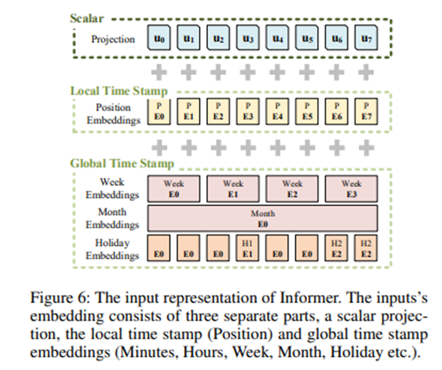
Local time stamp는 다음과 같이 positional embedding할 수 있다

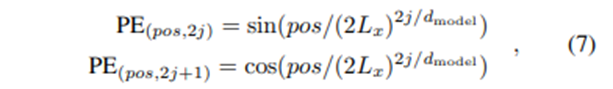
Where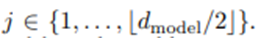

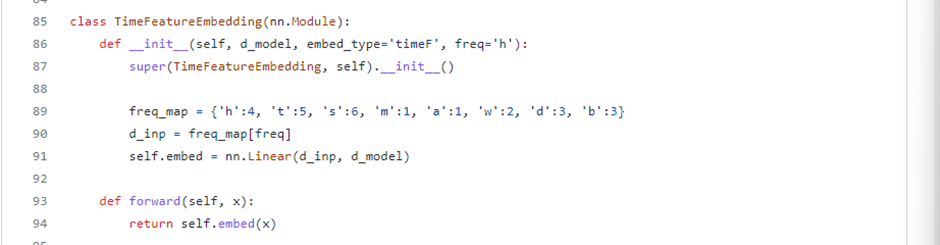
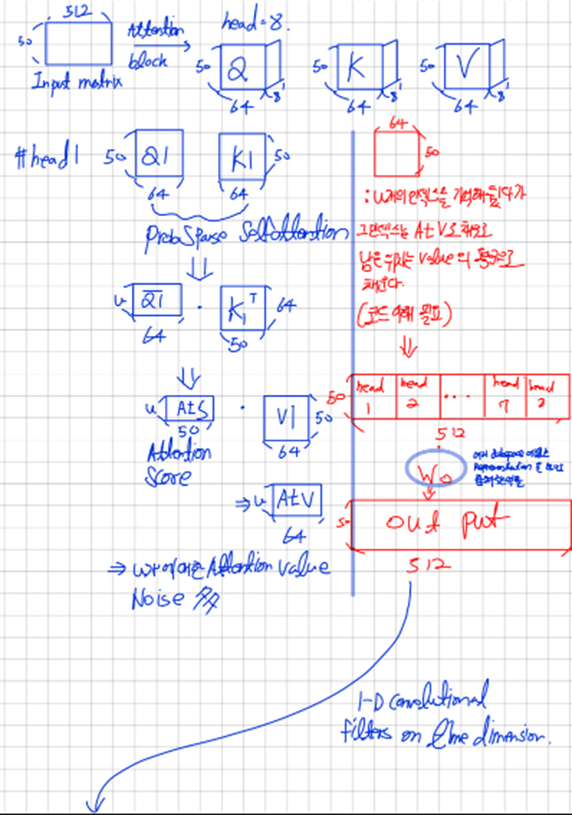
Github

또한 우리는 시계열 데이터 Input scalar의 dimension을 1-D convolutional filters(kernel width=3,stride=1) 를 통해 projection 시켜서 사용한다

출처

따라서 우리는 Scalar x를 convolution network를 통해 512차원의 벡터로 바꿨다(by padding)

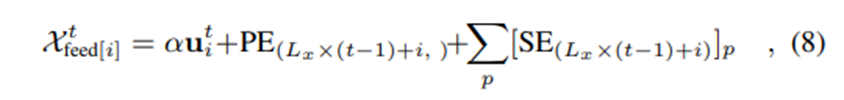
Where ⅈ∈{1,⋯,L_x }, and alpha is the factor balancing the magnitude between the scalar projection and local/global embeddings. 우리는 sequence input이 normalizing 됐다면 alpha=1을 추천한다

Methodology

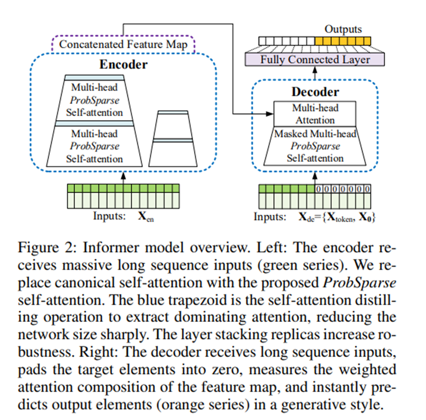
우리가 제안하는 Informer는 encoder-decoder architecture를 사용한다
Efficient Self-attention Mechanism
일반적인 Self-attention은 다음과 같이 정의된다

Transofmer review
$A(Q,K,V) = Softmax(QK’/sqrt(d))V ( ‘=transpose )$
$Where, QϵR^{L_Q Xd}, KϵR^{L_K Xd}, VϵR^{L_V Xd}$ and d is input dimension

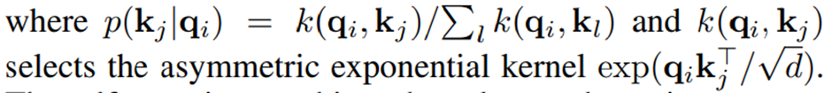
i번째 query의 attention은 다음과 같이 kernel function(여기서는 dot-product로 정의)을 통해 확률형태로 정의된다

(원래 self attention을 하는 과정을 가중평균의 관점에서 해석한 식)

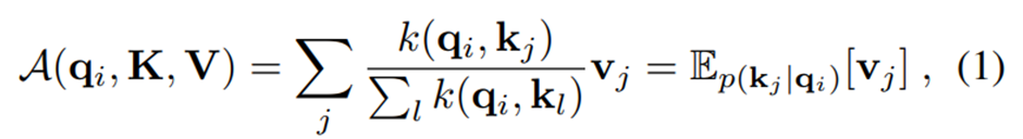
self-attention을 계산할 때는 Quadratic한( O(L_Q L_K ) ) time dot-product computation와 memory usage가 필요하다.
→이는 예측능력을 향상시키는 데에 있어 주된 문제점이다

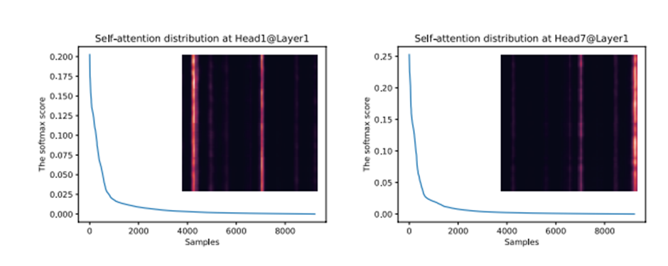
attention-score는 Sparsity(희소성)을 갖는다( 여기서 Sparsity는 의미 있는 값이 몇가지 없고 나머지는 다 0에 가까운 값이라는 의미)
따라서 이전의 연구자들은 Forecasting Performance의 변함이 거의 없이 어떻게 하면 좋은 attention score만 잘 선택할 수 있을까 고민을 했다
하지만 그들은 모든 multi-head self-attention에 같은 방식을 사용함으로써 추가적인 개선을 해내지 못했고 heuristic한 method를 사용했다

Sparsity한 self-attention score는 long tail distribution형태인데 이는 몇가지의 dot-product pairs만 major attention에 기여를 하고 다른 pairs들은 trivial한 attention(별 의미가 없는 attention)을 갖는다 이는 곧 어떻게 그들을 구분할 수 있는지에 대한 질문으로 이어진다

XAI를 공부할때 attention score를 attribution score로 볼 수 있음을 확인했다. 추후 XAI에 대해서 또 따로 올리겠다(word 50pg 정도 분량이라 시간이 좀 필요하다)

Query Sparsity Measurement
위에서 본 Eq.(1)은 i번째 query의 attention 계산 과정을 설명하고 있다
우리는 dominant한 attention score를 가지는 query-key pair는 attention score의 분포가 uniform distribution($q(k_j|q_i)=1/L_k$)와 떨어져 있을 것임을 알 수있다

Time Series는 매우 많은 시점들이 하나의 시점에 영향을 주고 있다고 생각할 수 있다. 물론 자기자신과의 관계성도 높게 나올 것 이지만 이외에도 관련 있는 것이 매우 많을 것이고 따라서 대부분의 시점에 대해서는 관계성이 낮게 나올테지만 특정시점에 대해서는 관계성이 높게 나올 것이다

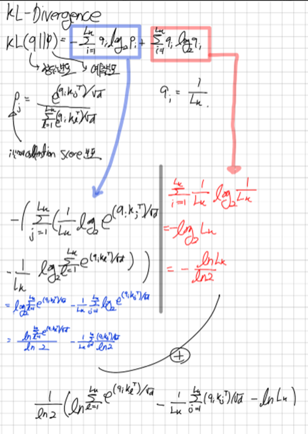
우리는 이런 분포 p , q사이의 Likeness를 측정하는 방법으로 KL divergence를 사용 할 것이다.KLDIVERGENCE MY BLOG

우리는 여기서 상수를 drop해서 i-th query’s sparsity measurement를 다음과 같이 쓸 수 있다(Query가 얼마나 Sparse한지 측정하는 지표 M)

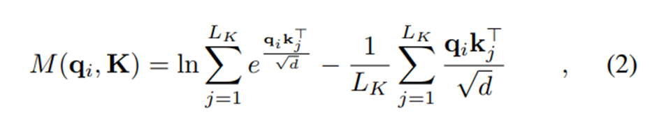
식 유도 (q = 정답분포, p = 예측분포)

ProbSparse Self-attention
위에서 계산한 query’s sparsity measurement에서 top u개[예측분포와 정답 분포사이의 유사도가 잘 맞지 않는 것들]의 query들을 포함하는 matrix를 $\bar Q$ Sparse Matrix라고 하고 ProbSparse Self-attention은 다음과 같이 계산한다

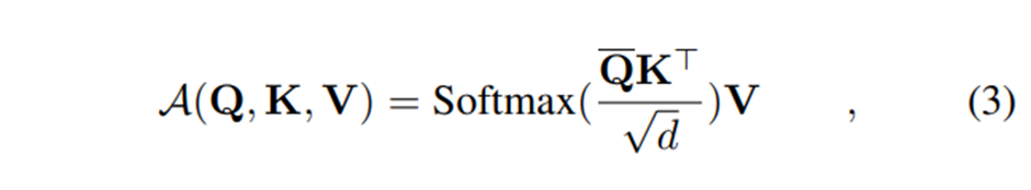
이때 $u = c ∘ln(L_Q)$ 이고 이때 c는 constant sampling factor로써 우리가 조절하는 조절자(hyperparameter)이다

ProbSparse Self-attention을 계산함으로써 우리는 $O(ln(L_Q))$ 만큼의 쿼리에 대해서만 dot-product연산만 하면 되고 $O(L_Kln(L_Q))$ 의 memory를 사용한다
Multi-head의 관점에서 각각의 head에 대해서 다른 query-key pairs를 생성하고 결과에서 정보손실을 피하게 된다.
하지만 모든 query에 대해 query’s sparsity measurement( $M(q_i,K)$)를 계산하기 위해서는 우리는
각각의 dot-product pairs의 계산이 필요하다 이는 Quadratic한 계산비용($O(L_K⁡*L_Q)$)이 필요하다
게다가 Log-Sum-Exp(LSE) operation은 수치적인 안정성 문제가 있다
이것이 동기가 돼서 우리는 효과적으로 query’s sparsity measurement를 얻기 위해 경험적인 근사방법(empirical approximation)을 제안한다.

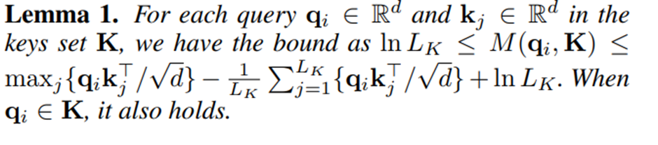
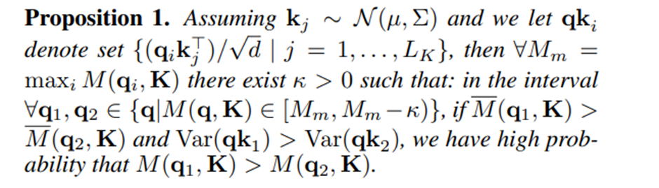
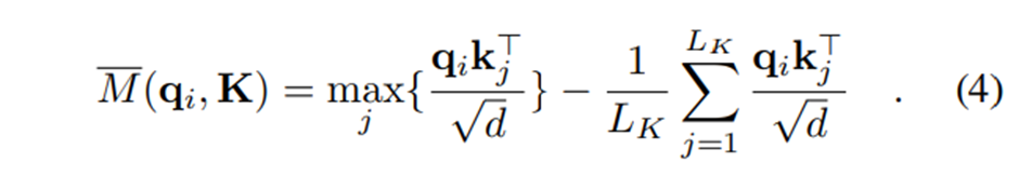
Lemma1에 의해서 M의 최대 최솟값을 제한하고 아래의 M(bar)를 query’s sparsity measurement 경험적인 근사값으로 사용한다
Proposition1은 M(bar)가 M을 대표할 수 있음을 보이고 동시에 모든 query에 key를 계산한 것과 모든 query의 Sampling된 key를 통해 계산한 query’s sparsity measurement(M) 계산 결과(순서)가 동일함을 나타낸다

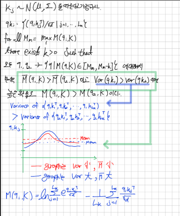
• $\bar M$은 Max에서 Mean을 빼는 것이기 때문에 파란색 분포가 빨간색 분포보다 크다.
  

$\bar M$를 얻기 위해서 $O(L_k L_Q)$ 만큼의 연산이 필요했지만 이는 Key를 $ln L_K$만큼 random하게 뽑아서 모든 Q와의 계산으로 Sample Score를 얻음으로써 해결한다 따라서 $O(L_Q ln L_K)$의 복잡도로 $\bar M$를 계산한다 그후 Top-u개의 query를 뽑아 $\bar Q$ 를 얻어낸다
아래는 ProbSparse self-attention의 알고리즘을 나타낸다

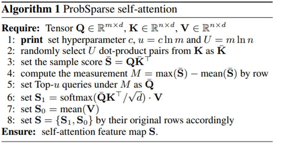
위 알고리즘을 통해 우리는
$ln ⁡L_k$ 개만큼의 Key를 뽑아서 $\bar K$ 를 만들고 이 Key(bar)와 Query들의 pair의 개수 $U=L_Q ln⁡L_k$
이렇게 sampling된 key 이용해서 $\bar M$ 를 계산하는 것을 알 수있다
우리는 $\bar M$를 사용하면서 안에 있는 max-operator가 zero value에 대해 덜 민감하고 수치적으로 안정시켰다 (LSE를 사용하지 않았기 때문)

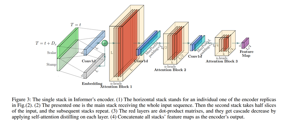
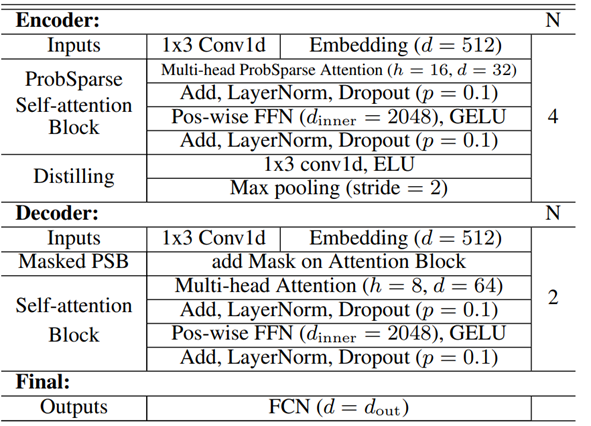
Encoder: Allowing for Processing Longer Sequential Inputs under the Memory Usage Limitation

Encoder는 long sequence input에 대해 robust한 long-range dependency를 추출하도록 디자인됐다.
Input representation과정이후 우리는 Scalar는 Conv1d Time stamp(global/local)는 LinearLayer를 통과하여 이를 더함으로써 t번째 Sequence input $χ^t$ 를 matrix 형태인 $X_{ⅇn}^t∈R^{L_x×ⅆ_{model}}$ 로 바뀌었다

다시 설명하면 위의 그림에서 확인할 수 있듯이 아까 input representation과정에서 우리의 Input scalar $x^t$ 를 1-D convolutional filter(kernel width=3, stride=1)인 필터로 $u^t$ (d_model dimension=512) 로 바꿨다

이를 우리가 train 하고 싶은 시간 간격 t=50(설명을 위해 내가 설정한 시간)에 대해서 실행하면 50x512(Lx×ⅆ{model}) 크기의 행렬로 바뀔 것이다
또 우리는 Local time stamp와 global time stamp를 각각 encoding과정을 통해서 Lx×ⅆ_model 의 크기로 되고 이들을 더하는 과정을 거쳐서 우리는 입력 데이터 행렬 x{en}로 만든다

Self-attention Distilling

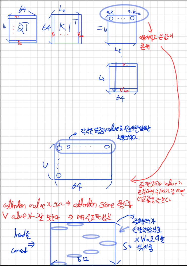
• (보라색 파란색 초록색 그림에 해당하는 설명)

ProbSparse self-attention mechanism의 자연스러운 결과로써 encoder의 feature map은 value V의 combination을 갖는다
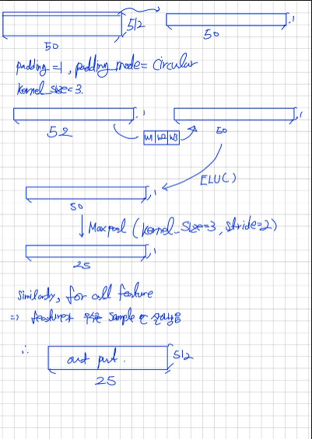
우리는 distilling operation의 convolution과정을 통해 특정 시간을 평활화(smoothing)하는 과정 뒤에 maxpooling과정을 통해 대표값을 하나 뽑는 과정을 거칠 것이다 이과정에서 Input의 시간차원$(L_x)$를 많이 깎는다
우리의 j 번째 layer에서 j+1번째 layer로 가는 distilling procedure는 다음과 같다

$[⋅]_{AB}$는 Attention block을 나타내고 이는 Multi-head ProbSparse self attention과 필요한 작업들을 포함하고 있다

Attention작업 도식화

<수정>
섞는다는 표현은 반은 맞고 반은 틀린 표현인데 Training이 가능한 가중치를 곱해줌으로써 중요한 정보와 덜 중요한 정보들의 가중치를 조절하면서 최적의 정보를 갖는 행을 만들어 내겠다는 의미이다

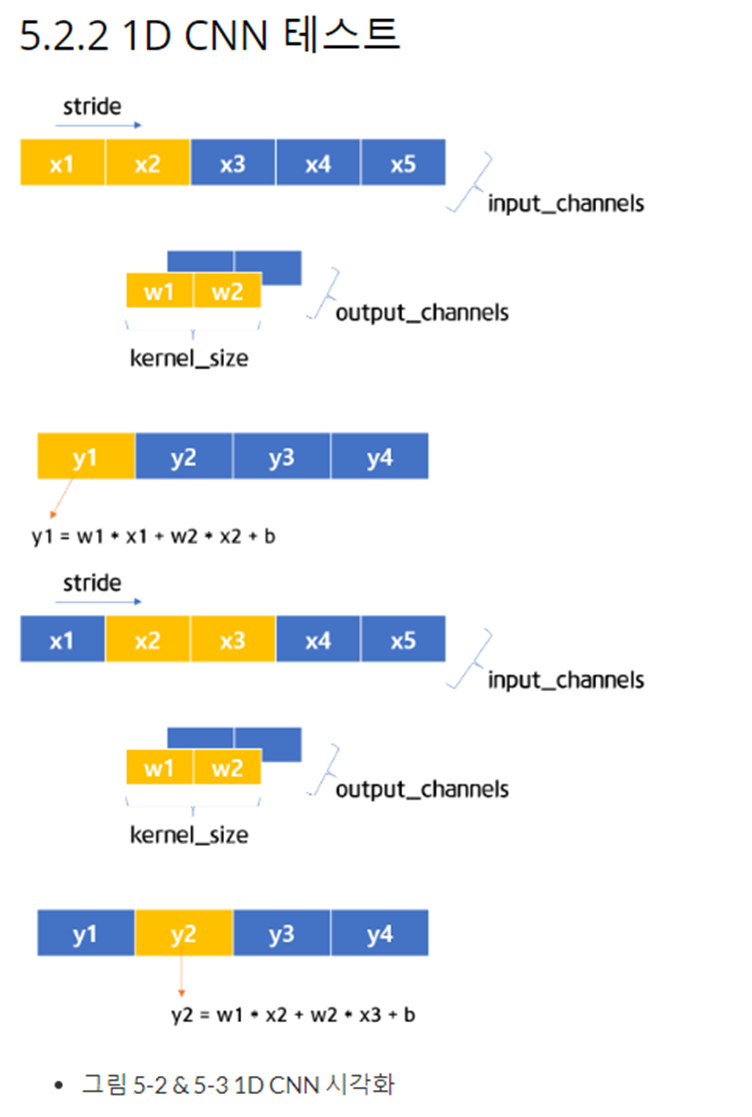
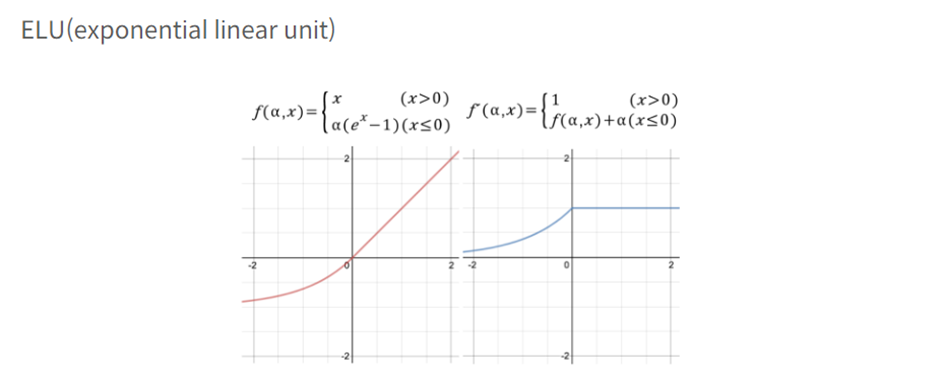
Where Conv1d(⋅) 는 1-D convolutional filters(kernel width=3, padding=1,padding_mode=circular) 을 time dimension 에 대해서 실시하고 ELU(⋅) activation function을 거친다
Conv1d를 통해 각 Feature별로 Time Series의 흐름을 뽑아내는 작업을 거친다(Smoothing 같은 과정)

이후 maxpooling(kernel_size=3, stride=2)를 통해서 ProbSparse self-attention을 거쳐서 나온 output의 각 Feature별로 주요한 정보흐름을 Capture해낸다
이후 같은 과정 반복한다 그러면 우리의 총 메모리 사용량은
$0((2-ε)LlogL$)으로 줄어들고 이는 self-attention computation complexity에 해당하는 메모리 LlogL이 $2-\epsilon$만큼 필요하다는 것이다 -> J개의 stacking layer에 대한 memory bottleneck 문제를 해결한 것이다( = Layer를 쌓아도 문제가 없다는 의미)
$cf. (1+1/2+1/4+1/8+⋯)≈(2-ε)$

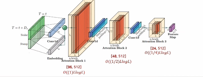
위의 과정의 도식화

Multi Encoder

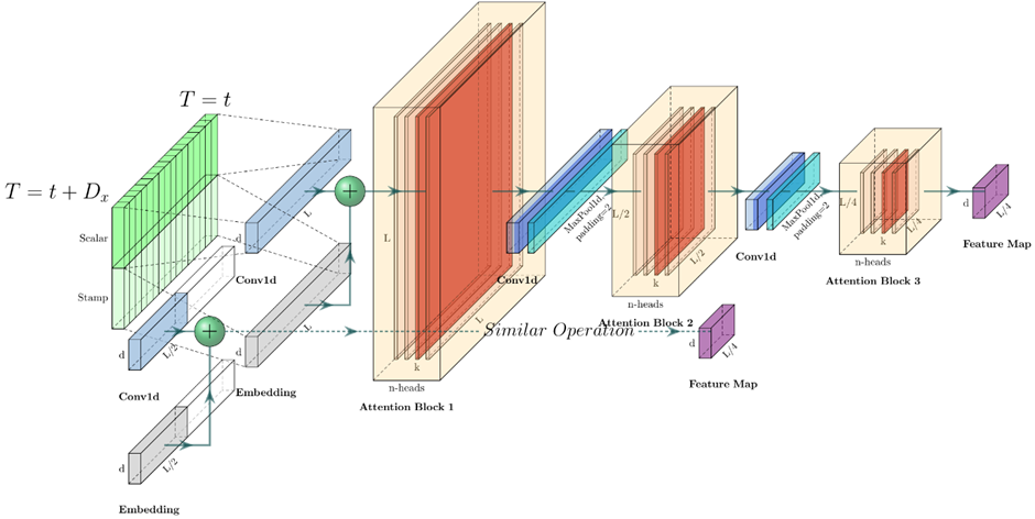
Distilling operation의 robustness를 강화하기 위해서 우리는 마지막 시점으로부터 Input의 크기를 절반만큼 줄인 main stack의 replicas를 만들고 layer를 하나 줄임으로써 output dimension을 맞춰 주었다
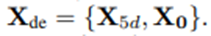
이후 이렇게 만든 모든 stack들의 output을 concatenate시켜서 encoder의 final hidden representation을 만들어 낸다

이렇게 Multi Encoder를 쓰는 것은 Residual Connection과 비슷한 개념이라고 생각하면 된다
우리가 만약에 하나의 Encoder만 쓰게 되면 입력데이터가 Encoding과정을 거친 후 어떤 편향을 갖고 Decoder에 입력 될 수 있다 따라서 우리는 Layer를 하나 덜 쓴 Encoder의 Output을 내서 깊은 Layer의 Feature Map을 붙여서 사용함으로써 더 깊은 Layer를 사용한 Encoding의 결과값의 편향이 영향을 크게 미치지 못하도록 조절해주는 영향을 한다
Concat을 시켜서 Decoder에 입력하면 시점이 꼬이지 않나? 라는 질문에는 시점정보 또한 하나의 숫자로 벡터안에 더해져 있으니 W_k, W_v라는 가중치가 이들의 시점이 꼬이지 않도록 잘 학습할 것을 기대한다

원문
To enhance the robustness of the distilling operation, we build replicas of the main stack with halving inputs, and progressively decrease the number of self-attention distilling layers by dropping one layer at a time, like a pyramid in Fig.(2), such that their output dimension is aligned. Thus, we concatenate all the stacks’ outputs and have the final hidden representation of encoder

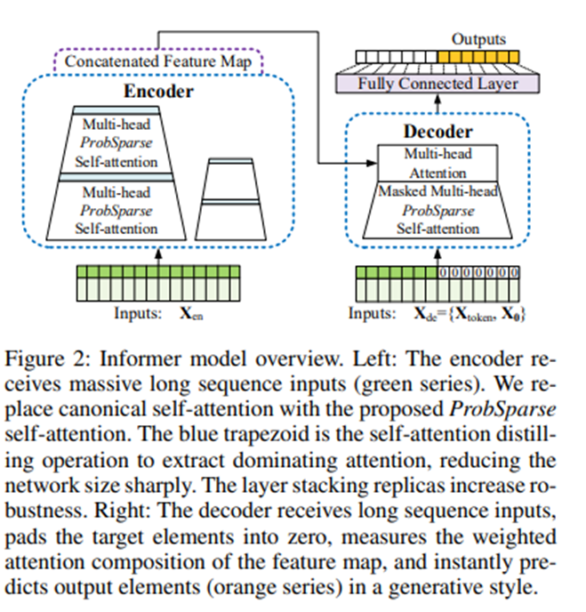
Decoder: Generating Long Sequential Outputs Through One Forward Procedure

One Forward Procedure이 중요하다.
Generative Inference는 Reculsively하게 결과를 생성하는 것이 아니고 한번에 Forward로 결과를 만들어내는 것을 말한다.

Informer의 decoder는 Standard decoder 구조를 사용한다
그리고 이 decoder는 두개의 동일한 multi head attention layer의 stack으로 구성됐다
하지만 우리는 generative inference를 쓰고 있는데 이는 long prediction에서 speed plunge(급락)현상을 개선시켜준다
우리는 decoder에 다음과 같은 벡터들을 feed시킨다

Where $X_{token}^t\in\mathbb{R}^{L_{token}\times d_{model}}$ 은 start token이고
$X_0^t\in\mathbb{R}^{L_y\times d_{model}}$는 target sequence에 대한 placeholder, scalar는 0으로 set되고 시간정보만 가지고 있다

Masked Multi-head ProbSparse Self-attention

Decoder에서는 Masked multi-head attention에 ProbSparse self-attention이 적용 된다
이는 특정시점의 예측을 미래시점 정보의 참여로부터 막는 역할을 한다
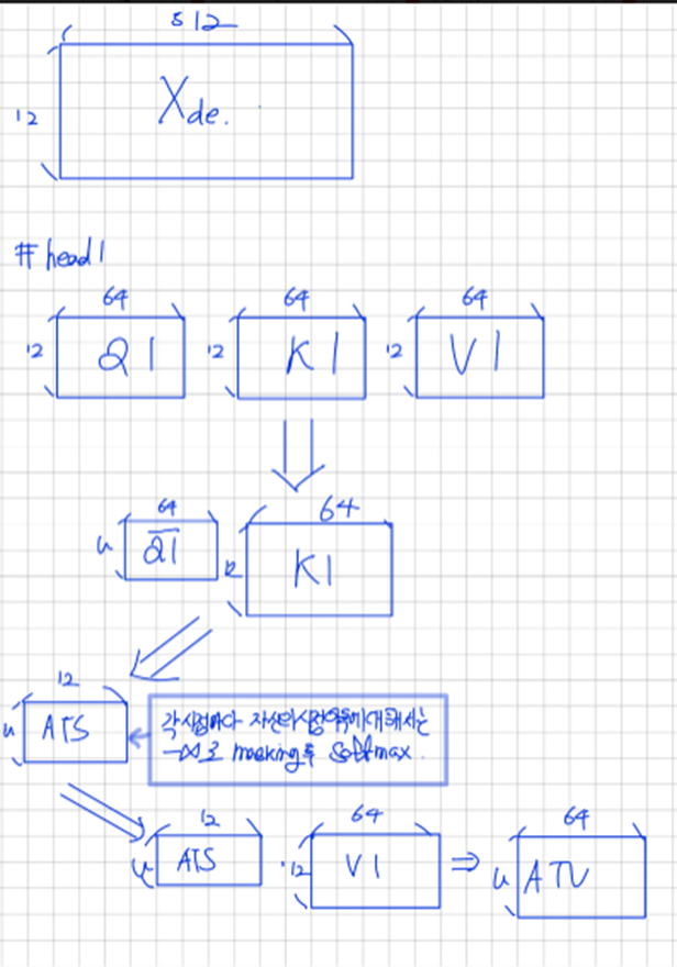
이후 multi-head attention을 거친 이후에 fully connected layer을 통과해서 최종 output을 얻는다

Generative Inference

Start token(sos)는 NLP의 dynamic decoding에서 효과적으로 적용된다 우리는 이 대신에
$L_{token}$ 길이의 sequence를 input sequence안에서 뽑아서 사용한다
예를 들어 168 point의 예측을 만든다면 우리는 target sequence 전에 알려진 5일을 start token으로 사용한다
따라서 decoder의 입력되는 값은
다음과 같다

Decoder Process

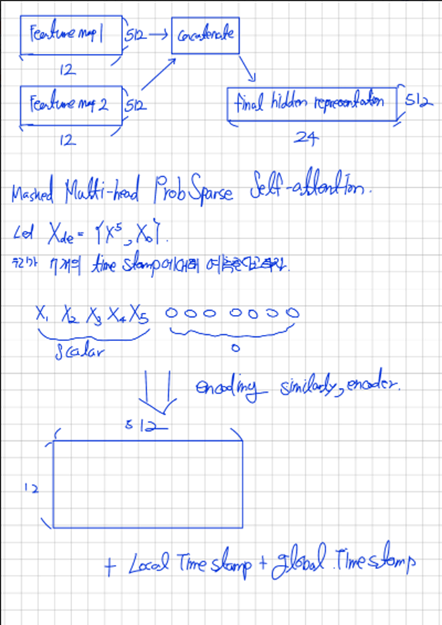
ATS: Attention Score
ATV: Attention Vector

Key와 Value는 Encoder의 hidden output

전체 구조

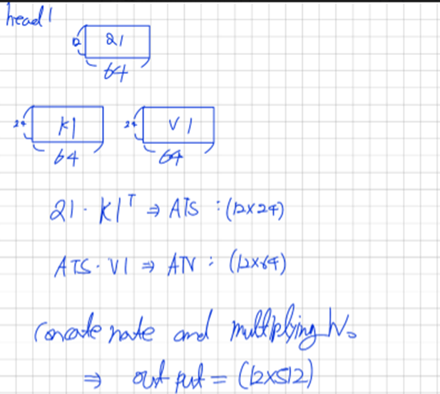
이렇게 만든 M.M.P.S output은 우리가 알고 싶은 것과 관계한 정보(이전 전체시점 정보)가 담겨져 있음
이를 Key와의 대조과정을 거치고 Value를 곱한다
여기서 Key의 각 행은 전체시간에 대한 어떤 흐름을 담고 있고 이 키와 Query(최근 시점 정보)를 대조한다