🎲[AI] Logistic Regression

해당 글은 FastCampus - '[skill-up] 처음부터 시작하는 딥러닝 유치원 강의를 듣고,
추가 학습한 내용을 덧붙여 작성하였습니다.

---

1. Logistic Regression

• 이진 분류(Binary Classification) 문제에 초점을 맞춘다
  어떻게 ? → Linear Regression + Sigmoid Function
• Logistic Regression: 선형 회귀 결과를 시그모이드 함수에 넣어 확률로 변환하고,
  그 확률로 분류를 수행하는 모델
• 시그모이드 출력값을 확률값 P(y|x)으로 생각할 수 있음
• Logistic == 로지스틱 함수(Logistic function) == Sigmoid function
• 이름은 Regression이지만 사실은 이진 분류(Binary clssification) 문제
  

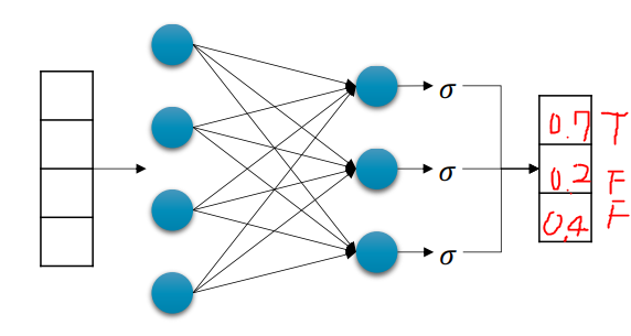
y_hat = σ(xW + b) 
True if y_hat >= 0.5 else False

Regression vs Classification

항목	회귀 (Regression)	분류 (Classification)
출력	실수 값 벡터	범주형 값
손실 함수	MSE Loss	BCE / Cross Entropy
마지막 계층	Linear	Sigmoid / Softmax
예	연봉 예측	감염 여부 예측

---

2. Sigmoid & Hypoerbolic Tangent Function

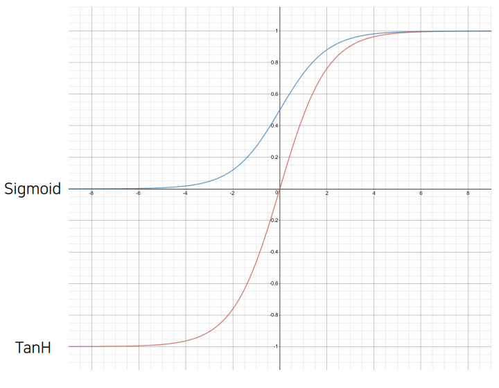
• σ(x) = $1 \over 1 + e^{-x}$ → 출력값을 0과 1 사이의 값으로 변환
  Tanh(x) = $e^{x} - e^{-x} \over e^{x} + e^{-x}$ → 출력값을 -1과 1 사이의 값으로 변환
• 로지스틱 회귀에서는 활성화 함수로 Sigmoid 사용
• 이 값을 확률 P(y|x)로 해석 가능

---

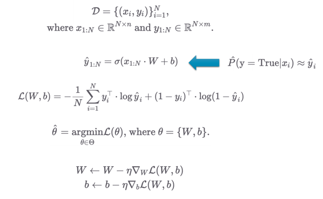
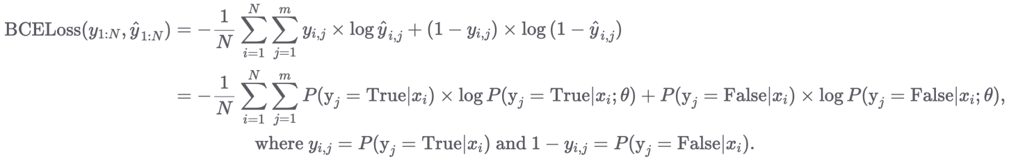
3. Loss function: Binary Cross Entropy (BCE)

• 실제 정답이 1이라면 확률 ŷ는 1에 가깝게
  실제 정답이 0이라면 확률 ŷ는 0에 가깝게 학습되도록 유도하는 손실 함수

• $BCE(y_{1:N},ŷ_{1:N}) = - \frac{1}{N} \sum (y_i^T \log(ŷ_i) + (1 - y_i)^T \log(1 - ŷ_i))$
  $x_i ϵ R^n$, $y_i ϵ \{0,1\}^m$

• 수식의 앞 부분은 True만을 살리는 부분, 뒷 부분은 False만을 살리는 부분
  → - 가 앞에 있으므로 minimize 함수가 되는 것
  

• 시그모이드의 출력은 0과 1 사이의 확률이므로 BCE 손실함수 사용 (MSE를 써도 풀리긴 하지만 최적화 X)

• BCELoss같은 경우에는 확률/통계, 정보 이론과 밀접한 관련이 있음

---

4. 파라미터 최적화

• 마찬가지로 손실 함수를 W, b에 대해 미분하여 기울기 계산
  
• 손실함수 detail
  

---

5. Pytorch 실습 코드

$θ ← θ - η▽_θL(θ)$ x 200,000 iterations
$y = f(x)$
$x ∈ R^{569 X 10}$
$y ∈ R^{569 X 1}$

$D = {(x_i, y_i)}^{N=569}_{i=1}$
$ŷ = f_θ(x) = σ(x*W + b)$
$θ = \{W, b\}$
$W ∈ R^{10X1}$
$b ∈ R^{1X1}$
$L(θ) = - \frac{1}{N} \sum (y_i^T \log(ŷ_i) + (1 - y_i)^T \log(1 - ŷ_i))$

import pandas as pd
import seaborn as sns
import matplotlib.pyplot as plt
import torch
import torch.nn as nn
import torch.nn.functional as F
import torch.optim as optim
from sklearn.datasets import load_breast_cancer
cancer = load_breast_cancer()

# print(cancer.DESCR)

df = pd.DataFrame(cancer.data, columns=cancer.feature_names)
df['class'] = cancer.target

# df.tail()

### Pair plot with mean features
# sns.pairplot(df[['class'] + list(df.columns[:10])])
# plt.show()

### Pair plot with std features
# sns.pairplot(df[['class'] + list(df.columns[10:20])])
# plt.show()

### Pair plot with worst features
# sns.pairplot(df[['class'] + list(df.columns[20:30])])
# plt.show()

### Select features

cols = ["mean radius", "mean texture",
        "mean smoothness", "mean compactness", "mean concave points",
        "worst radius", "worst texture",
        "worst smoothness", "worst compactness", "worst concave points",
        "class"]

for c in cols[:-1]:
    sns.histplot(df, x=c, hue=cols[-1], bins=50, stat='probability')
    plt.show()

## Train Model with PyTorch

data = torch.from_numpy(df[cols].values).float()

print(data.shape)

x = data[:, :-1]
y = data[:, -1:]

print(x.shape, y.shape)

n_epochs = 200000
learning_rate = 1e-2
print_interval = 10000

class MyModel(nn.Module): #nn.Module을 상속받아서 나만의 custom 모델 만들기
    
    def __init__(self, input_dim, output_dim):
        self.input_dim = input_dim
        self.output_dim = output_dim
        
        super().__init__()
        
        self.linear = nn.Linear(input_dim, output_dim)
        self.act = nn.Sigmoid()
        
    def forward(self, x):
        # |x| = (batch_size, input_dim)
        # |y| = (batch_size, output_dim)
        y = self.act(self.linear(x))
        
        return y

model = MyModel(input_dim=x.size(-1),
                output_dim=y.size(-1))
crit = nn.BCELoss() # Define BCELoss instead of MSELoss.

optimizer = optim.SGD(model.parameters(), # 나중에 기울기 구할 parameter들 등록
                      lr=learning_rate)

for i in range(n_epochs):
    y_hat = model(x)
    loss = crit(y_hat, y)
    
    optimizer.zero_grad()
    loss.backward() # model.parameters()에 포함된 모든 텐서(W, b, ...)에 대해 gradient (∂loss/∂parameter)를 자동 계산
    
    optimizer.step()
    
    if (i + 1) % print_interval == 0:
        print('Epoch %d: loss=%.4e' % (i + 1, loss))

correct_cnt = (y == (y_hat > .5)).sum()
total_cnt = float(y.size(0))

print('Accuracy: %.4f' % (correct_cnt / total_cnt))

df = pd.DataFrame(torch.cat([y, y_hat], dim=1).detach().numpy(),
                  columns=["y", "y_hat"])

sns.histplot(df, x='y_hat', hue='y', bins=50, stat='probability')
plt.show()

---