🎲[AI] Overfitting & Underfitting

해당 글은 FastCampus - '[skill-up] 처음부터 시작하는 딥러닝 유치원 강의를 듣고,
추가 학습한 내용을 덧붙여 작성하였습니다.

---

1. Overfitting이란?

• 우리의 목표: 학습 데이터뿐 아니라 새로운 데이터(unseen data)에 대해서도 잘 예측하는 모델
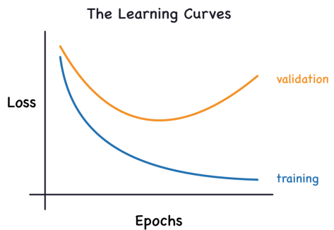
  → 즉, Training error를 최소화 하는 것이 최종 목표가 아님
• Overfitting: Training Error (학습 데이터 오차)보다 Generalization Error (일반화 오차)가 현저히 높아지는 현상
  • 학습 데이터의 bias와 noise까지 과도하게 학습함
  • Overfitting 현상이 꼭 나쁜 것은 아님
    → 모델의 capacity가 충분한지 확인하는 하나의 방법 (물론 확인 후에는 overfitting 해결 必)
    

---

2. Underfitting이란?

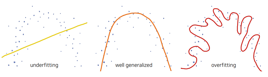
• 모델의 capacity(depth, width)가 부족해 training error 가 충분히 낮지 않은 상태

---

3. Overfitting vs Underfitting

용어	설명
Overfitting	불필요한 패턴까지 학습
Underfitting	데이터의 기본 패턴조차 학습하지 못함
Well-generalized	학습 데이터와 새로운 데이터 모두에서 좋은 성능

---

4. Overfitting을 막기 위한 Validation Set 활용

• train/validation/test 데이터를 random하게 분할 e.g. 6:2:2
• validaiton, test set은 절대 학습에 사용 X (Scaling fit 단계에서도 마찬가지임!)
• training set으로 학습, 매 epoch가 끝나면 validation set으로 generalization 성능 추정
• training error만 낮고 validation error가 높다면 overfitting 신호
• Early Stopping: 일정 epoch 동안 validation loss 개선 없으면 학습 중단

데이터셋	목적
Training Set	파라미터 학습
Validation Set	generalization 및 hyperparameter 검증
Test Set	최종 모델 및 알고리즘 검증

---

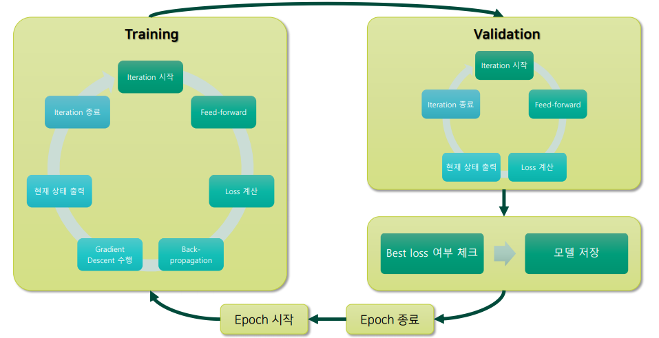
5. Typical Training Procedure

1. 데이터 분할
2. train set으로 feed-forward, loss 계산, SGD 수행
3. training error 계산
4. validation set으로 feed-forward, loss 계산 (학습은 X)
5. validation error 계산
6. best 모델 저장 (최저 validation loss 기준)
7. test set으로 최종 평가

---

6. Pytorch 실습 코드

# Split into Train / Valid / Test set

## Load Dataset from sklearn

import numpy as np
import pandas as pd
import seaborn as sns
import matplotlib.pyplot as plt

from sklearn.preprocessing import StandardScaler

from sklearn.datasets import fetch_california_housing
california = fetch_california_housing()

df = pd.DataFrame(california.data, columns=california.feature_names)
df["Target"] = california.target
df.tail()

## Convert to PyTorch Tensor

import torch
import torch.nn as nn
import torch.nn.functional as F
import torch.optim as optim

data = torch.from_numpy(df.values).float()

x = data[:, :-1]
y = data[:, -1:]

print(x.size(), y.size())

# Train / Valid / Test ratio
ratios = [.6, .2, .2]

train_cnt = int(data.size(0) * ratios[0])
valid_cnt = int(data.size(0) * ratios[1])
test_cnt = data.size(0) - train_cnt - valid_cnt
cnts = [train_cnt, valid_cnt, test_cnt]

print("Train %d / Valid %d / Test %d samples." % (train_cnt, valid_cnt, test_cnt))

# Shuffle before split.
indices = torch.randperm(data.size(0))
x = torch.index_select(x, dim=0, index=indices)
y = torch.index_select(y, dim=0, index=indices)

# Split train, valid and test set with each count.
x = list(x.split(cnts, dim=0))
y = y.split(cnts, dim=0)

for x_i, y_i in zip(x, y):
    print(x_i.size(), y_i.size())

## Preprocessing

scaler = StandardScaler()
scaler.fit(x[0].numpy()) # You must fit with train data only.

x[0] = torch.from_numpy(scaler.transform(x[0].numpy())).float()
x[1] = torch.from_numpy(scaler.transform(x[1].numpy())).float()
x[2] = torch.from_numpy(scaler.transform(x[2].numpy())).float()

df = pd.DataFrame(x[0].numpy(), columns=california.feature_names)
df.tail()

## Build Model & Optimizer

model = nn.Sequential(
    nn.Linear(x[0].size(-1), 6),
    nn.LeakyReLU(),
    nn.Linear(6, 5),
    nn.LeakyReLU(),
    nn.Linear(5, 4),
    nn.LeakyReLU(),
    nn.Linear(4, 3),
    nn.LeakyReLU(),
    nn.Linear(3, y[0].size(-1)),
)

model

optimizer = optim.Adam(model.parameters())

## Train

n_epochs = 4000
batch_size = 256
print_interval = 100

from copy import deepcopy

lowest_loss = np.inf
best_model = None

early_stop = 100
lowest_epoch = np.inf

train_history, valid_history = [], []

for i in range(n_epochs):
    # Shuffle before mini-batch split.
    indices = torch.randperm(x[0].size(0))
    x_ = torch.index_select(x[0], dim=0, index=indices)
    y_ = torch.index_select(y[0], dim=0, index=indices)
    # |x_| = (total_size, input_dim)
    # |y_| = (total_size, output_dim)
    
    x_ = x_.split(batch_size, dim=0)
    y_ = y_.split(batch_size, dim=0)
    # |x_[i]| = (batch_size, input_dim)
    # |y_[i]| = (batch_size, output_dim)
    
    train_loss, valid_loss = 0, 0
    y_hat = []
    
    for x_i, y_i in zip(x_, y_):
        # |x_i| = |x_[i]|
        # |y_i| = |y_[i]|
        y_hat_i = model(x_i)
        loss = F.mse_loss(y_hat_i, y_i)

        optimizer.zero_grad()
        loss.backward()

        optimizer.step()        
        train_loss += float(loss)

    train_loss = train_loss / len(x_)

    # You need to declare to PYTORCH to stop build the computation graph.
    with torch.no_grad():
        # You don't need to shuffle the validation set.
        # Only split is needed.
        x_ = x[1].split(batch_size, dim=0)
        y_ = y[1].split(batch_size, dim=0)
        
        valid_loss = 0
        
        for x_i, y_i in zip(x_, y_):
            y_hat_i = model(x_i)
            loss = F.mse_loss(y_hat_i, y_i)
            
            valid_loss += loss
            
            y_hat += [y_hat_i]
            
    valid_loss = valid_loss / len(x_)
    
    # Log each loss to plot after training is done.
    train_history += [train_loss]
    valid_history += [valid_loss]
        
    if (i + 1) % print_interval == 0:
        print('Epoch %d: train loss=%.4e  valid_loss=%.4e  lowest_loss=%.4e' % (
            i + 1,
            train_loss,
            valid_loss,
            lowest_loss,
        ))
        
    if valid_loss <= lowest_loss:
        lowest_loss = valid_loss
        lowest_epoch = i
        
        # 'state_dict()' returns model weights as key-value.
        # Take a deep copy, if the valid loss is lowest ever.
        best_model = deepcopy(model.state_dict())
    else:
        if early_stop > 0 and lowest_epoch + early_stop < i + 1:
            print("There is no improvement during last %d epochs." % early_stop)
            break

print("The best validation loss from epoch %d: %.4e" % (lowest_epoch + 1, lowest_loss))

# Load best epoch's model.
model.load_state_dict(best_model)

## Loss History

plot_from = 10

plt.figure(figsize=(20, 10))
plt.grid(True)
plt.title("Train / Valid Loss History")
plt.plot(
    range(plot_from, len(train_history)), train_history[plot_from:],
    range(plot_from, len(valid_history)), valid_history[plot_from:],
)
plt.yscale('log')
plt.show()

## Let's see the result!

test_loss = 0
y_hat = []

with torch.no_grad():
    x_ = x[2].split(batch_size, dim=0)
    y_ = y[2].split(batch_size, dim=0)

    for x_i, y_i in zip(x_, y_):
        y_hat_i = model(x_i)
        loss = F.mse_loss(y_hat_i, y_i)

        test_loss += loss # Gradient is already detached.

        y_hat += [y_hat_i]

test_loss = test_loss / len(x_)
y_hat = torch.cat(y_hat, dim=0)

sorted_history = sorted(zip(train_history, valid_history),
                        key=lambda x: x[1])

print("Train loss: %.4e" % sorted_history[0][0])
print("Valid loss: %.4e" % sorted_history[0][1])
print("Test loss: %.4e" % test_loss)

df = pd.DataFrame(torch.cat([y[2], y_hat], dim=1).detach().numpy(),
                  columns=["y", "y_hat"])

sns.pairplot(df, height=5)
plt.show()