Generative Modeling by Estimating Gradients of the Data Distribution

새로운 형태의 Generative Model 을 제안한 Song & Ermon (2019) 논문을 리뷰해 보았다.

Abstract

이 논문에서는, score matching 를 통해 추정된 데이터 분포의 gradient를 이용한 Langevin dynamic 을 기반으로 새로운 ‘생성 모델’ 을 소개한다. 차원이 낮은 데이터의 경우, 그 gradient 를 추정하기 어렵거나 잘못된 값으로 정의될 수 있기에, 데이터에 서로 다른 Gaussian noise 를 추가해 ‘혼란’ 시키고, 대응되는 score 를 추정한다. Sampling 의 경우, 이 논문에서는 annealed 된 Langevin dynamic 을 제안한다. Sampling process 가 저점 noise 를 감소시키며 원본 data 에 가까워지면서 대응되는 gradient 를 계산한다. 논문에서 제안한 프레임워크에서, 모델의 구조는 flexible 하며 adversarial 한 method 를 적용하거나 학습을 하는 과정에서 sampling 이 필요하지 않고, 모델 비교를 위한 목적 함수를 유도한다. 제안한 모델은 MNIST, CelebA, CIFAR-10 데이터셋에 대한 GAN 의 결과와 비교할 만한 sample 을 생성하며, CIFAR-10 데이터셋에 대해서는 Inception score 8.87 이라는 결과 (SOTA)를 얻어냈다. 더 나아가, 모델이 image inpainting 을 통해 이미지로부터 효과적인 representation 을 학습한다는 것을 보여준다.

1. Introduction

생성 모델 (Generative model) 은 머신러닝 분야에서 많이 응용되고 있다. 응용 분야 중 일부를 나열해 보자면, 1) 고화질 이미지 생성 2) 음성 및 음악 합성 3) Semi-supervised learning 의 성능 향상 4) 비정상적인 데이터(anomalies) 및 상반되는 데이터(adversarial data) 감지 5) 모방학습 (Imitation learning) 이 있다. 최근에 제시되는 응용 사례는 두 가지 접근 1) likelihood 기반 방법 2) GAN 을 기반으로 한다. 전자의 경우 목적 함수로 log-likelihood 를 사용하며, 후자의 경우 모델이 예측한 데이터의 분포와 실제 데이터 분포 간의 f-divergence 또는 integral probability 로 정의된 목적 함수의 값을 최소화시키는 방향으로 학습이 진행된다.

비록 likelihood 기반 방법 및 GAN 이 generative model 분야에서 좋은 성능을 나타냈지만, 한계점을 가지고 있다. 예를 들어, 학습을 위해서는 likelihood 를 사용하는 모델 (e.g. 자기회귀 (autoregressive) 모델, flow model)의 경우 정규화된 확률 모델을 만들기 위한 특수한 모델 구조가 필요하며, EBM (energy-based model) 의 경우 contrastive divergence, VAE 의 경우 대리 손실함수 (surrogate loss) 가 필요하다. GAN 의 경우 이러한 한계점들 중 일부는 극복하지만, 경쟁적인 학습 과정으로 인해 학습이 불안정할 수 있다. Noise contrastive estimation 과 minimum probability flow 와 같이 생성 모델을 구축을 위한 training object 역시 존재하지만, 이러한 방법들은 낮은 차원의 데이터에 대해서만 잘 적용된다는 한계점을 지니고 있다.

이 논문에서는, 생성 모델을 구현하는 새로운 원리를 소개한다. 이는 logarithmic data density 의 Stein score 로 부터의 추정 및 샘플링에 기반한다. 즉 입력 데이터에 대한 log-density 가 가장 빠르게 증가하는 방향을 가리키는 벡터장을 이용하는 것이다. 데이터로부터 이러한 벡터장을 학습하기 위해, score matching 방법으로 학습된 인공 신경망을 사용한다. 이후 Langevin dynamic 을 이용한 sampling 으로부터 sample 을 생성한다. 임의로 생성된 (초기) sample 값을 추정된 벡터장을 따라 높은 density 를 가지는 영역으로 업데이트 하며, 원본 data 에 가까운 sample 을 생성하는 방향으로 이동하게 된다. 그러나, 이 방법에는 크게 2가지의 문제점이 있다. 첫 번째로, 만약 데이터의 차원이 낮다면 (실세계의 많은 데이터셋이 이러한 경우를 따른다), data point 주위의 영역에서 score 가 정의되지 않는 경우가 생기고 결과적으로 score matching 으로부터 올바른 score estimator 를 제공받지 못한다. 두 번째로, 데이터 밀도가 낮은 영역에서의 데이터가 희소한 점은 (즉, 대부분의 데이터가 존재하는 manifold 로부터 ‘멀리 떨어진’ 데이터들의 경우) score estimation 의 정확도를 감소시키며 Langevin dynamics sampling 과정을 느려지게 한다. 대부분의 경우 Langevin dynamics 는 데이터 분포에 대해 밀도가 낮은 영역에서 초기화되므로, 이 영역에서 부정확한 score estimation 이 일어난다면 샘플링 과정에 악영향을 미치게 된다. 더 나아가, 여러 분포가 mixing 되어 각 분포의 최빈값 간의 거리가 먼 경우 역시 sampling 이 어려워진다.

이러한 두 가지 문제점을 극복하기 위해, 다양한 크기의 gaussian noise 를 data 에 추가해 data 분포에 혼란을 가져다주는 방법을 제안한다. Random noise 를 추가함으로써 데이터 분포가 낮은 차원에만 머물지 않게 한다. 큰 noise 의 경우 기존 data 분포 에 대해 낮은 밀도 영역 상의 sample 을 생성하므로, score estimation 과정이 잘 일어날 수 있게 한다. 결정적으로, noise level 에 의존하는 단일 score network 를 학습시켜 모든 크기(magnitude, level)의 noise 에 대한 score 를 추정한다. 그 다음으로, Langevin dynamics 의 annealed version 을 제안한다. Annealed version 의 경우, 가장 높은 noise level 에 대한 score 를 초기값으로 해, sampling 결과와 원본 데이터가 구분될 수 없을 때 까지 noise level 을 점점 감소시키며 score estimation 과정을 수행한다.

논문에서 제안한 접근 방식은 몇 가지 중요한 특징을 가진다. 첫 번째로, training object 를 최적화시키는 과정에서 adversarial training, MCMC sampling, 또는 다른 근사 기법이 필요하지 않으며, score network 설계를 위한 독특한 구조 또는 별도의 제약이 필요하지 않고, 대부분의 신경망 매개화 기법에 대해 training object 를 계산할 수 있다 (tractable). 또한 training object 를 이용해, 같은 데이터셋에 대한 서로 다른 모델의 성능을 정량적으로 비교할 수도 있다. 논문에서는 제안된 방식이 MNIST, CelebA, CIFAR-10 데이터셋에 대해 유효함을 보이며 최근에 제안된 likelihood-base model 및 GAN 의 결과와 비교할 만한 sample 을 생성함을 보인다. 특히 CIFAR-10 데이터셋에 대해서는, unconditional 생성 모델에 대한 inception score 8.87 의 값을 얻어 SOTA 를 갱신하고, FID score 25.32 를 얻었다. 마지막으로 image inpainting 을 통해 데이터에 대한 meaningful representation 을 학습함을 보인다.

2. Score-based generative modeling

학습에 사용한 데이터셋이 분포 $p_{data}\left(\mathbf{x}\right)$ 을 따르는 i.i.d sample $\{\mathbf{x}_i\ \in\R^D\}_{i=1}^N$ 라고 가정하자. 확률 밀도 $p\left(\mathbf{x}\right)$ 에 대한 Score 는 다음과 같이 정의한다.

Score network 는 parameter $\theta$에 대해 매개화된 인공 신경망 $s_\mathbf{\theta}:\R^D\rightarrow\R^D$ 이며, $p_{data}\left(\mathbf{x}\right)$ 의 score 를 추정하도록 학습된다. Modeling 의 목표는 주어진 분포 $\mathbf{p}_{\mathbf{data}}\left(\mathbf{x}\right)$ 로부터 새로운 sample 을 생성하는 모델을 dataset 을 이용해 학습시키는 것이다. 이와 같이 score 에 기반하는 생성 모델에 대한 프레임워크는 1) score matching 과 2) Langevin dynamics 라는 요소를 가진다.

본문에서, ‘데이터 분포에 대한 밀도가 낮은 영역’ 은 데이터가 적게 분포하는 영역, ‘밀도가 높은 영역’ 은 데이터가 많이 분포하는 영역을 의미한다.

2.1. Score matching for score estimation

Score matching 은 알 수 없는 데이터 분포 (unknown data distribution) 으로부터 추출된 i.i.d sample 에 의존하는 비 정규화된 통계 모델을 학습시키기 위해 제안된 것이 그 시초이다. 그러나 논문에서는 score matching 을 score estimation 이라는 다른 용도로써 사용한다. Score matching 을 이용해, $p_{data}\left(\mathbf{x}\right)$ 를 추정하는 별도의 모델 없이 score network $s_\mathbf{\theta}\left(\mathbf{x}\right)$ 가 $\nabla_\mathbf{x}\log{p_{data}\left(\mathbf{x}\right)}$ 를 바로 추정하도록 직접적으로 학습시킬 수 있다. 이는 기존에 score matching 이 활용되던 방식과는 다르게, 고차원의 gradient 로 인한 추가적인 연산을 줄이기 위해 EBM 의 gradient 를 score network 로써 사용하지 않는다. 최소화 시키고자 하는 object 는

로, 이는 아래 식과 동치이다. (단, $\nabla_\mathbf{x}s_\mathbf{\theta}\left(\mathbf{x}\right)$ 는 $s_\mathbf{\theta}\left(\mathbf{x}\right)$ 의 야코비 행렬

증명은 아래와 같다.

---

을 전개해 보자. 나오는 항들 중

는 상수이다. 따라서 training object 에서 omit 할 수 있다.

항의 경우, integration by parts 에 의해

와 동치이다. 여기에

를 더하고 상수 1/2 을 omit 시키면, Training object 는

와 동치이다.

---

연산 과정에서 $\mathbb{E}_{p_{data}\left(\mathbf{x}\right)}$ 는 데이터셋을 통해 비교적 쉽게 구할 수 있지만, $\text{tr}\left(\nabla_\mathbf{x}s_\mathbf{\theta}\left(\mathbf{x}\right)\right)$ 는 구하는 과정에서 문제가 발생하는데, 고차원의 데이터에 대해서 score matching 이 적용되기 어려워진다. 따라서 large scale 에 대한 score matching 을 위한 두 가지 방법에 대해 논의한다.

2.1.1. Denoising score matching : estimates the scores of perturbed data

Denoising score matching 은 trace 를 계산하지 않는 변형된 score matching 이다. 우선, 데이터 point $\mathbf{x}$ 에 사전에 정의된 noise distribution $q_\sigma\left(\tilde{\mathbf{x}}\middle|\mathbf{x}\right)$ 를 이용해 noise 를 추가한다 (perturb). Noise 가 추가된 데이터의 분포 $q_\sigma\left(\tilde{\mathbf{x}}\right)$ 는

가 되고, 이에 대해 score matching 을 진행한다. Training object 는 다음과 같이 변형된다.

식을 전개하고 적분 형태로 변형해 다음 식을 유도할 수 있다.

이는 2.1. 에서 정의한 training object 와 $\nabla_{\tilde{\mathbf{x}}}\log{q_\sigma\left(\tilde{\mathbf{x}}\right)}$ 부분에서 차이가 있다 ($\nabla_\mathbf{x}\log{p_{data}\left(\mathbf{x}\right)}$ 와 다름). 이 때, 위 식을 최소화하는 optimal score network $s_{\mathbf{\theta}^\star}\left(\mathbf{x}\right)$ 는,

를 (대부분의 경우) 만족한다. 두 식의 차이를 없애기 위해서는

가 만족될 정도로 noise 가 충분히 작아야 한다.

2.1.2. Sliced score matching : estimates the scores of unperturbed data

Sliced score matching 의 경우
$\text{tr}\left(\nabla_\mathbf{x}s_\mathbf{\theta}\left(\mathbf{x}\right)\right)$ 값을 추정하기 위해 적절한 projection 을 사용한다. Random vector (e.g. multivariate standard normal distribution)의 분포를 $p_\mathbf{v}$ 라고 하면, ($\mathbf{v}$ 에 대한 정사영을 생각해 보면) training object 는

와 동치이다. 증명은 다음과 같다.

---

우선,

이다. 또한,

가 성립한다. 만약 $\mathbf{v}$가 multivariate standard normal distribution 을 따른다면,

이므로

가 성립한다.

---

$\mathbf{v}^T\nabla_\mathbf{x}s_\mathbf{\theta}\left(\mathbf{x}\right)\mathbf{v}$ 항은 forward mode 의 자동 미분을 통해 효율적으로 계산 가능하다. Denoising score matching 이 perturbed 된 data 에 대해 추정을 한다면, sliced score matching 은 unperturbed data 에 대한 score estimation 을 제공한다. 그러나, sliced score matching 은 자동미분 과정으로 인해 denoising score matching 보다 약 4배의 연산이 더 필요하다.

2.2. Sampling with Langevin dynamics

Langevin dynamics 는 score function $\nabla_\mathbf{x}\log{p\left(\mathbf{x}\right)}$ 만을 이용해 확률밀도함수 $p\left(\mathbf{x}\right)$ 로부터 샘플을 생성할 수 있다. $\forall\epsilon>\ 0$, 사전 분포 $\pi$ (e.g. uniform noise) 에 대한 초기값 $\tilde{\mathbf{x}}_0\sim\pi\left(\mathbf{x}\right)$, $\mathbf{z}_t\sim\mathcal{N}\left(0,I\right)$ 에 대해, Langevin method 는 재귀적으로 다음과 같이 값을 계산한다.

$\epsilon\rightarrow0,\ T\ \rightarrow\ \infty$ 일 때 $\tilde{\mathbf{x}}_t\ \sim p\left(\mathbf{x}\right)$ 가 성립한다. 즉 일부 조건 하에, $\tilde{\mathbf{x}}_t$가 $p\left(\mathbf{x}\right)$ 로부터 추출한 sample 이 되는 경우에 해당한다.

$\epsilon>\ 0,\ T\ <\ \infty$ 일 때 위 식의 오차를 보정하기 위해 Metropolis-Hastings update 가 필요하나, 대부분의 경우 실제로는 무시 가능하다. 논문에서는 $\epsilon$ 이 작고 $T$가 큰 경우 오차가 무시 가능하다고 가정한다.

2.2.에 나타난 과정을 이용해서 샘플링 하는 과정은 단지 $\nabla_\mathbf{x}\log{p\left(\mathbf{x}\right)}$ 만을 필요로 한다. 따라서 $p_{data}\left(\mathbf{x}\right)$ 로부터 샘플을 얻기 위해서는, 우선 $\mathbf{s}_\mathbf{\theta}\left(\mathbf{x}\right)\simeq \mathbf{\nabla}_\mathbf{x}\log{p_{data}\left(\mathbf{x}\right)}$ 를 만족하는 score network 를 학습시키고, 두 번째로 Langevin dynamics 를 이용해 $\mathbf{s}_\mathbf{\theta}\left(\mathbf{x}\right)$ 로부터 유사하게 sampling 을 진행한다.

이것이 논문에서 제안한 score-based generative modeling 프레임워크의 핵심 아이디어이다.

3. Challenges of score-based generative modeling

3절에서는 2절에서 소개한 아이디어를 보다 구체적으로 분석한다. 이 아이디어를 적용하는 데 있어서, 2개의 제약점이 있다는 것을 밝힌다.

3.1. The manifold hypothesis

Manifold hypothesis 는 실세계의 데이터가 고차원 공간 (ambient space)에 내장된 낮은 차원의 manifold 에 존재한다는 점을 나타낸다. 이 가설은 여러 데이터셋에 대해 경험적으로 성립하며, manifold learning 의 시초가 되었다. Manifold hypothesis 하에, 논문에서 제안한 score-based generative model 은 2가지 문제점을 마주친다. 1) 정의한 score $\nabla_\mathbf{x}\log{p_{data}\left(\mathbf{x}\right)}$ 는 ambient space 에서 계산된 gradient 이므로, 만약 $\mathbf{x}$가 낮은 차원의 manifold 에 존재한다면 gradient 가 정의되지 않는다. 2) 식

은 데이터가 전체 공간에 분포할 때만 적절한 score estimator 를 제공하며, 데이터가 낮은 차원에 밀집해 있는 경우 올바르지 않은 score estimating 이 일어난다.

Figure 1. 에서 manifold hypothesis 가 score estimation 에 가져다주는 악영향을 볼 수 있다.

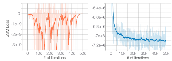
Figure 1. SSM (Sliced score matching) loss with respect to iterations.
Source : Song & Ermon. (2019)

Figure 1. 은 CIFAR-10 에 대한 score 를 추정하기 위해 ResNet 을 학습시키는 과정을 나타낸다. Left figure 는 데이터에 noise 가 추가되지 않은 경우, right figure 는 데이터에 $\mathcal{N}\left(0,{0.01}^2\right)$ 을 따르는 noise 가 추가된 경우를 나타낸다.Score matching 의 경우 Sliced score matching 을 사용하였다. Left side 의 경우 loss 가 처음에는 감소하지만 이후 불규칙하게 증가와 감소를 반복하며, Right side 처럼 작은 gaussian noise 를 데이터에 추가한 경우 loss 는 점점 작은 값으로 수렴한다. 여기서 추가한 noise 는 $\mathcal{N}\left(0,{0.01}^2\right)$ 를 따르는 값으로 인간의 눈으로는 구분이 불가능 할 정도이며, [0, 1]의 픽셀값을 가지는 이미지 기준으로도 매우 작은 값이다.

3.2. Low data density regions

데이터 밀도가 낮은 영역에서의 데이터가 희소한 점은, score matching 을 통한 score estimation 과정과 Langevin dynamic 을 이용한 sampling 과정에 어려움을 야기한다.

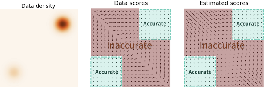
Estimated scores are only accurate in high density regions.
Figure source : Yang Song, “Generative Modeling by Estimating Gradients of the Data Distribution”, 2021.05.05, https://yang-song.net/blog/2021/score/

3.2.1. Inaccurate score estimation with score matching

데이터 밀도가 낮은 영역의 경우, data sample 의 수가 부족하므로 score matching 이 score 를 정확하게 estimate 를 하지 못한다. Score matching 을 통해

의 값을 최소화 하고자 함을 다시 생각해 보자 (2.1. 절 참고). 실제 과정에서는 $p_{data}\left(\mathbf{x}\right)$ 로부터 추출된 i.i.d sample $\{\mathbf{x}_i\}_{i=1}^N$ 을 이용해 기댓값을 추정한다. 그렇다면 다음과 같은 영역 $\mathcal{R}\in\mathbf{R}^D$ 를 고려해 보자.

대부분의 경우,

이며, score matching 을 통해 $\mathbf{x}\in\mathcal{R}$ 에 대한 $\nabla_\mathbf{x}\log{p_{data}\left(\mathbf{x}\right)}$ 의 값을 추정하기에는 데이터 sample 이 충분하지 않다.

이러한 문제점을 증명하기 위해, Toy experiment 를 시행하였다. 이 실험에서 데이터의 분포 $p_{data}$ 는 mixture of Gaussian 으로 두었다.

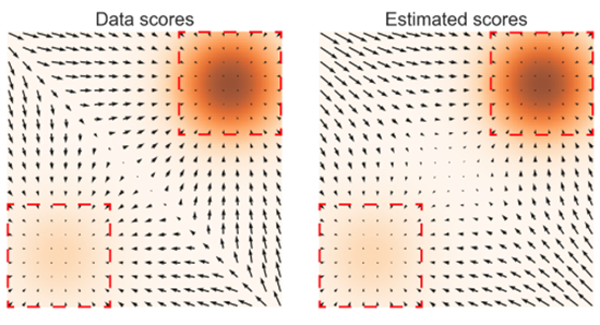
우선 $p_{data}\left(\mathbf{x}\right)$ 에 대한 score function 과 density function 을 도시하면 아래 Figure 와 같다.

Figure source : Yang Song, “Generative Modeling by Estimating Gradients of the Data Distribution”, 2021.05.05, https://yang-song.net/blog/2021/score/

Toy experiment 의 결과는 Figure 2. 와 같다.

Figure 2. Result of Toy experiment.
Source : Song & Ermon. (2019)

Figure 2. 에서, 주황색 부분은 $p_{data}$의 분포를 나타낸다. 어두운 영역은 데이터의 밀도가 높은 부분을 나타내며, 빨간색 점선 테두리의 직사각형은 $\nabla_\mathbf{x}\log{p_{data}\left(\mathbf{x}\right)}\simeq s_\mathbf{\theta}\left(\mathbf{x}\right)$ 가 성립하는 부분을 나타낸다. Left figures 는 $\nabla_\mathbf{x}\log{p_{data}\left(\mathbf{x}\right)}$ 를 도시한 결과이며, right figure 는 $s_\mathbf{\theta}\left(\mathbf{x}\right)$ 를 도시한 결과이다. Figure 2. 에서 나타나듯이, 데이터 밀도가 높은 영역, 즉 $p_{data}$ 의 최빈값과 근접한 부분에서만 score estimation 이 정확 (reliable) 하다.

3.2.2. Slow mixing of Langevin dynamics

데이터 분포의 두 최빈값이 밀도가 데이터 낮은 영역에 의해 분리될 경우, Langevin dynamics 는 두 최빈값에 대한 상대적인 가중치를 적절한 시간 내에 산출하지 못하며, 결과적으로 sampling 의 결과가 true distribution 으로 수렴하지 못한다.

결합 분포 $p_{data}\left(\mathbf{x}\right)=\pi p_1\left(\mathbf{x}\right)+\left(1-\pi\right)p_2\left(\mathbf{x}\right)$ 를 생각해 보자. $\pi\in\left(0,1\right)$ 이고, $p_1\left(\mathbf{x}\right)$와 $p_2\left(\mathbf{x}\right)$는 disjoint support 를 가지는 정규화된 분포이다. Support $p_1\left(\mathbf{x}\right)$ 만을 고려할 경우,

가 성립하고, support $p_2\left(\mathbf{x}\right)$ 만을 고려할 경우,

가 성립한다. 두 경우 모두, score $\nabla_\mathbf{x}\log{p_{data}\left(\mathbf{x}\right)}$ 는 $\pi$에 의존하지 않는다. 2.2. 절에 나와 있듯, Langevin dynamic 은 $p_{data}\left(\mathbf{x}\right)$ 로부터 sampling 을 위해 $\nabla_\mathbf{x}\log{p_{data}\left(\mathbf{x}\right)}$ 를 필요로 하므로, 얻어진 sample 들 역시 $\pi$에 의존하지 않는다. 실제로는, 서로 다른 최빈값이 approximately disjoint support 를 가지더라도 이러한 분석이 성립한다. 이 경우 이론적으로는 Langevin dynamic 을 통해 올바른 sample 을 생성할 수 있지만, mixing 을 위해서는 매우 작은 step size와 많은 step 이 필요하다.

이 분석이 타당함을 보이기 위해, 논문에서는 3.2.1.절에서 사용한 mixture of Gaussian 과 동일한 분포에 대해 Langevin dynamics 를 적용해 sampling 을 수행하며, 그 결과는 Figure 3. 와 같다. Figure 3. (b) 는 3.2.2. 에서 설명하고 있는 경우인 “데이터 분포의 두 최빈값이 밀도가 데이터 낮은 영역에 의해 분리될 경우” 에 해당하며, (a) 와 비교해 보았을 때 분석에 의한 결과와 동일하게 Langevin dynamics 가 두 최빈값의 밀도를 잘못 추정함을 알 수 있다.

Figure 3. Mixture of Gaussian 으로부터의 sampling. 3가지의 서로 다른 방법을 사용하였다. (a) 분포로부터 직접적인 sampling (b) Langevin dynamics 를 이용한 sampling (c) annealed Langevin dynamics 를 이용한 sampling. (b) 의 결과로부터, 데이터 분포의 두 최빈값으로부터 상대적인 weight 를 잘못 추정함을 볼 수 있다. (c) 의 경우, 앞서 소개된 Langevin dynamics 의 annealed version 을 이용한 것으로 weight 를 올바르게 추정함을 볼 수 있다.
Source : Song & Ermon. (2019)

4. Noise Conditional Score Networks : learning and inference

데이터를 random Gaussian noise 를 이용해 perturb 시키는 것이 데이터 분포가 score-based gradient modeling 을 잘 따르게 함을 확인하였다. 첫 번째로, Gaussian noise 분포의 support (지지집합)은 (모든 차원을 포함하는) 전체 공간이므로, perturb 된 데이터 분포의 경우 낮은 차원의 공간에만 국한되어 있지 않고, 이는 3.1. 에 제시된 manifold hypothesis 로부터 발생되는 문제점을 방지하고 score estimation 이 잘 일어날 수 있게 한다. 두 번째로, 큰 gaussian noise 는 원래의 (unperturbed) 데이터 분포에 대해 밀도가 낮은 영역을 채워주는 효과가 있고, 따라서 score estimation 이 더욱 정확해 진다. 더 나아가, 여러 noise level 을 사용함으로써 true data distribution 에 수렴하는 noise-perturbed distribution 의 집합을 얻을 수 있다. 이렇게 모인 distribution 과 simulated annealing, annealed importance sampling 을 사용해 다봉분포에 대한 Langevin dynamics 의 mixing rate 를 증가시킬 수 있다.

위 내용에 기반해, 논문에서는 score-based generative modeling 을 다음과 같은 방법을 이용해 발전시키고자 한다. 1) 다양한 level 의 noise 를 통한 data perturbing 2) 단일 conditional score network 학습을 통해, 모든 noise level 에 대응되는 score 를 동시에 추정하는 것. 학습이 끝난 후 샘플링을 위해 Langevin dynamics 를 사용할 때 가장 큰 noise 에 대한 score 를 초기값으로 사용하고, noise level 을 점차 감소시킨다. 이는 perturbed 된 데이터가 원본 데이터와 거의 구분될 수 없을 정도의 수준으로 noise level 을 낮추는 데 있어서 높은 noise level 의 이점을 유연하게 전달해준다. 지금부터는 score network 의 구조, training object, 그리고 Langevin dynamics 의 annealing 에 대해 보다 구체적으로 설명한다.

4.1. Noise Conditional Score Networks

$\{\sigma_i\}_{i=1}^L$ 을

을 만족하는 양의 기하급수라고 하자. Perturbed data distribution 을 나타내는 $q_\sigma\left(\mathbf{x}\right)$ 를 다음과 같이 정의하자.

Noise levels $\{\sigma_i\}_{i=1}^L$ 은 다음과 같이 선택한다.

$\sigma_1$ : 3. 에 제시된 문제점들을 완화시키기에 충분히 큰 값
$\sigma_L$ : data 에 미치는 영향을 최소화하는 충분히 작은 값

모든 perturbed data 분포에 대한 score 를 공동으로 추정하게끔 Noise Conditional Score Network (NCSN) $s_\mathbf{\theta}$ 를 학습시킨다. 즉,

가 성립하게끔 학습을 진행한다. $\mathbf{x}\in\mathbf{R}^D$ 일 때 $s_\mathbf{\theta}\left(\mathbf{x},\sigma\right)\in\mathbf{R}^D$ 이다.

Likelihood 에 기반한 생성 모델 및 GAN 과 유사하게, 좋은 품질의 sample 을 생성에 있어서 모델 구조 설계는 매우 중요하다. 이 연구에서는 이미지 생성에 유용한 구조에 주로 집중하며, 다른 응용 분야에 적용될 수 있는 구조들은 후속 연구로 남겨둔다. NCSN 의 출력값이 입력되는 이미지 $\mathbf{x}$ 와 동일한 shape 를 가지므로, 이미지의 dense prediction (e.g. 의미론적 분할) 에서 좋은 결과를 나타낸 모델 구조를 참고한다. 구현의 경우 U-Net 의 구조와 dilated/atrous convolution 의 구조를 결합한 모델을 사용한다. 더 나아가, NCSN 에 $\sigma_i$ 에 대한 conditioning 을 위해 변형된 conditional instance normalization 을 적용한다.

4.2. Learning NCSNs via score matching

NCSN 학습을 위해, 2.1. 에 소개된 sliced score matching 과 denoising score matching 모두를 사용할 수 있다. 논문에서는 더 빠르고 noise로 perturbed 된 데이터 분포에 대해 score 를 추정하는 denoising score matching 을 사용한다. 그러나, 실험적으로 봤을 때 sliced score matching 역시 denoising score matching 만큼 NCSN 을 잘 학습시킬 수 있다. Noise 의 분포가

이 되게끔 하고, 따라서,

가 성립한다. 주어진 $\sigma$에 대한 score matching object 는, 2.1. 절에서 유도한 바와 같이

위 식을 $\forall\sigma\in\{\sigma_i\}_{i=1}^L$ 에 대해 결합해 하나로 통일된 object 를 유도하면

여기서 $\lambda\left(\sigma_i\right)$ 는 양의 값으로 $\sigma_i$ 에 의존하는 계수 함수이다. $s_\mathbf{\theta}\left(\mathbf{x},\ \sigma\right)$ 의 capacity 가 충분히 크다고 가정하면, $\mathbf{s}_{\mathbf{\theta}^\star}\left(\mathbf{x},\ \mathbf{\sigma}\right)$ 가 $\mathbf{L}\left(\mathbf{\theta};\{\mathbf{\sigma}_\mathbf{i}\}_{\mathbf{i}=\mathbf{1}}^\mathbf{L}\right)$ 을 최소화 시키는 필요충분조건은 $\forall\mathbf{i}\ \in\{\mathbf{1},\ \mathbf{2},\ \cdots,\ \mathbf{L}\}$ 에 대해

를 만족하는 것이다.

함수 $\lambda$ 에는 다양한 선택지가 있다. 이상적인 경우는 모든 $\{\sigma_i\}_{i=1}^L$ 에 대해 $\lambda\left(\sigma_i\right)l\left(\mathbf{\theta};\sigma_i\right)$ 가 (대략적으로) 같은 크기를 가지는 것이다. 실험적으로 봤을 때 학습을 통해 score network 를 최적화 시킨 경우 근사적으로

가 성립한다. 이로부터, $\lambda\left(\sigma_i\right)l\left(\mathbf{\theta};\sigma_i\right)$ 가 $\sigma$에 의존하지 않게 하기 위해서는

로 두어야 함을 알 수 있다. 왜냐하면 이 경우

가 성립하고,

이므로 $\lambda\left(\sigma_i\right)l\left(\mathbf{\theta};\sigma_i\right)$ 의 값이 $\sigma$에 의존하지 않는다.

논문에서는 training object $\mathcal{L}\left(\mathbf{\theta};\{\sigma_i\}_{i=1}^L\right)$ 가 1) adversarial training 을 필요로 하지 않고 2) surrogate loss 을 사용하지 않으며 3) training 과정에서 sampling 이 필요하지 않음을 강조한다. 또한, $s_\mathbf{\theta}\left(\mathbf{x},\ \sigma\right)$ 가 tractable 해지기 위해 특별한 구조를 필요로 하지 않는다. 추가적으로, $\lambda$ 와 $\{\sigma_i\}_{i=1}^L$ 가 고정되어 있는 경우 서로 다른 NCSN 들을 정량적으로 비교하는 데에도 사용할 수 있다.

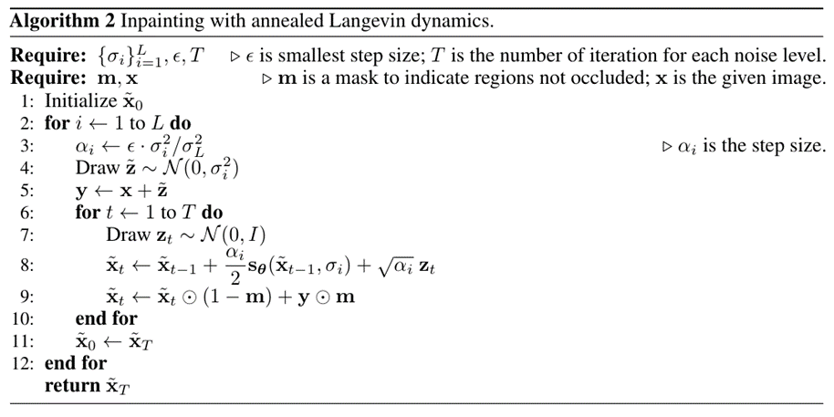
4.3. NCSN inference via annealed Langevin dynamics

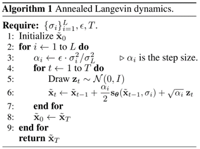
NCSN $s_\mathbf{\theta}\left(\mathbf{x},\ \sigma\right)$ 을 학습시킨 후, annealed Langevin dynamics 라는 sampling 기법을 적용한다. Algorithm 은 아래와 같다.

Algorithm for annealed Langevin dynamics.
Source : Song & Ermon. (2019)

사전에 정의된 분포 (e.g. uniform noise) 로부터 초기 sample $\tilde{\mathbf{x}_0}$을 얻는다. 이후 재귀적으로 sampling 을 진행하는데, $q_{\sigma_{i-1}}\left(\mathbf{x}\right)$ 를 초기 sample 로 하는 Langevin dynamics 를 이용해 $q_{\sigma_i}\left(\mathbf{x}\right)$ 를 얻는다 (총 $T$번 sampling). Noise level 이 감소할수록, step size $\alpha_i$ 역시 감소시킨다. 최종적으로, $q_{\sigma_L}\left(\mathbf{x}\right)$ 로부터 Langevin dynamics 를 이용해 $\sigma_L\simeq0$ 일 때 $p_{data}\left(\mathbf{x}\right)$ 와 가까운 sample 을 얻는다.

모든 분포 $\{q_{\sigma_i}\}_{i=1}^L$ 가 Gaussian noise 에 의해 perturb 되었으므로, 각각의 지지집합은 전체 (실수) 공간을 형성하며, manifold hypothesis 에서 발생하는 문제점을 방지해 score 가 잘 정의된다. $\sigma_1$ 이 충분히 크다면, 분포 $q_{\sigma_1}\left(\mathbf{x}\right)$ 의 밀도가 낮은 부분이 줄어들고, 최빈값은 비교적 가까워지게 된다 (less isolated). 이전에 논의된 바와 같이, 이러한 특징은 더욱 정확한 score estimate 를 가능하게 해 주며, mixing process 를 빠르게 해 준다. 따라서 Langevin dynamics 가 $q_{\sigma_1}\left(\mathbf{x}\right)$에 대한 좋은 sample 을 생성함을 알 수 있다. 이 때 생성된 sample 들은 분포 $q_{\sigma_1}\left(\mathbf{x}\right)$의 밀도가 높은 영역에서 추출되었을 가능성이 높으며, 이는 분포 $q_{\sigma_2}\left(\mathbf{x}\right)$에 대해서도 밀도가 높은 영역에 속할 가능성이 높음을 의미한다. Score estimation 과 Langevin dynamics 는 데이터 밀도가 높은 영역에서 더 좋은 결과를 만들어 내므로, $q_{\sigma_1}\left(\mathbf{x}\right)$으로부터 얻은 sample 은 $q_{\sigma_2}\left(\mathbf{x}\right)$에 대해 좋은 initial sample 로써 작용한다. 이러한 과정이 반복되어, $q_{\sigma_{i-1}}\left(\mathbf{x}\right)$은 $q_{\sigma_i}\left(\mathbf{x}\right)$를 얻기 위한 좋은 initial sample 이 되며, 결과적으로 $q_{\sigma_L}\left(\mathbf{x}\right)$ 으로부터 높은 quality 의 sample 을 얻을 수 있다.

Step size $\alpha_i$ 를 정하는 데에는 여러 가지 방법이 있다. 논문에서는 Langevin dynamics 의 SNR (Signal-to-Noise Ratio) 을 고정시켜 주기 위해 다음과 같이

설정하였다. 증명은 아래와 같다.

---

우선, SNR 은 다음과 같이 정의된다.

이 때,

여기서 $\alpha_i\propto\sigma_i^2$ 를 대입하면

이 때 4.2. 절에 기술된 것 처럼 score network 를 최적화 시킨 경우 근사적으로

가 성립함을 발견하였으므로, 결과적으로

가 성립한다. 즉 SNR 은 $\sigma_i$ 에 의존하지 않는 상수가 되는 것이다.

---

Annealed Langevin dynamics 의 타당성을 입증하기 위해, Toy example 실험을 시행하였다. $\{\sigma_i\}_{i=1}^L$ 는 기하급수로 정의하였으며, $L=10$, $\sigma_1=10$, $\sigma_{10}=0.1$ 로 두었다. 자세한 내용과 분석 결과는 Figure 3. 에 기재되어 있다.

요약하자면, score network 가 주어진 noise level $\sigma_i$ 에 대해 perturbed data 의 log-density 가 가장 빠르게 증가하는 방향 ($\nabla_\mathbf{x}\log{q_{\sigma_i}\left(\mathbf{x}\right)}$) 을 가리키게끔 학습된다. Sampling 과정에서는 이전 noise level 에서의 결과를 score network 가 가리키는 방향 (즉 원본 데이터 분포에 가까워지는 방향) 으로 이동시키고 noise $(z_t)$ 를 추가하면서 sampling 을 진행한다. 하나의 noise level 에 대해 sampling 은 총 $T$번 진행된다.

5. Experiments

5절에서는 NCSN 이 자주 사용되는 주요 이미지 dataset 에 대해 높은 품질의 sample 을 생성함을 보인다. 더 나아가, image inpainting 을 통해 NCSN 이 image 에 대한 적절한 representation 을 학습함을 보인다.

5.1. Setup

데이터셋으로는 MNIST, CelebA, CIFAR-10 을 사용한다. 모든 이미지들의 픽셀값은 [0, 1] 로 scaling 되었다. CelebA의 경우 중심부를 $140\ \times140$ size 로 잘라낸 후 $32\ \times32$ 로 resize 되었다. $\{\sigma_i\}_{i=1}^L$ 은 기하급수로 정의되었으며 $\sigma_1=1, \sigma_{10}=0.01, L=10$ 으로 두었다. $\sigma=0.01$인 Gaussian noise 는 인간의 눈으로는 거의 구분 불가능하다는 점을 참고하자. Annealed Langevin dynamics 에서는 $T=100$, $\epsilon=2\times{10}^{-5}$, 사전에 정의된 noise 분포로는 균등 분포(uniform) 를 사용하였다.

5.2. Image generation

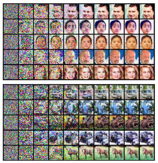
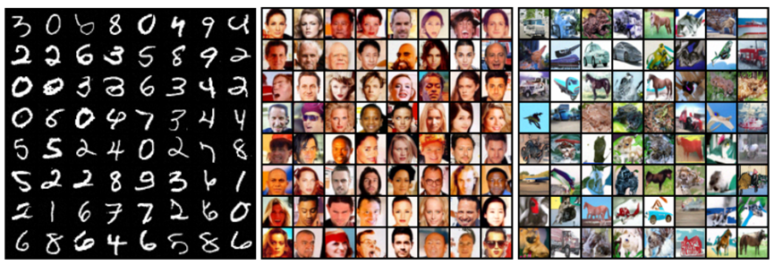
Figure 5. 는 각각 MNIST, CelebA, CIFAR-10 에 대해 annealed Langevin dynamics 를 통해 sampling 된 결과를 보여준다. Figure 5. 에서 볼 수 있듯이, NCSN 을 통해 생성된 이미지들은 최신 연구들에서 제안된 likelihood-based model 또는 GAN 보다 품질이 더 높거나 비교할 만하다. Intermediate sample 의 경우 Figure 4. 에 나타나 있다. 각 행은 각각의 sample 이 random noise 로부터 어떻게 생성되는지 그 과정을 나타낸다.

Figure 4. Annealed Langevin dynamics 의 intermediate sample.
Source : Song & Ermon. (2019)

Figure 5. Sampling result from NSCN (a) MNIST (b) CelebA (c) CIFAR-10
Source : Song & Ermon. (2019)

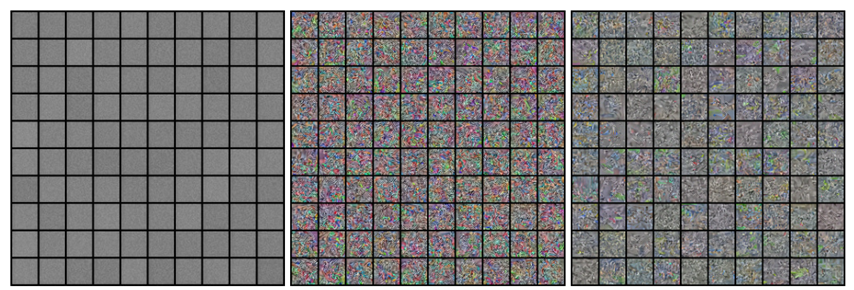
여러 noise level 에 대한 conditional score network 와 annealed Langevin dynamics 의 중요성을 시험해 보기 위해, baseline 모델과 NSCN의 결과를 비교한다. Baseline 모델은 하나의 noise level ($\sigma_1=0.01$) 만을 사용하며, Langevin dynamics 를 annealed version 이 아닌 vanilla version 을 사용한다. 비교 결과는 Figure 7. 에 나타나 있다. Baseline model 의 경우 제대로 된 sample 을 생성하지 못함을 확인할 수 있다.

Figure 7. Sampling result from baseline model (a) MNIST (b) CelebA (c) CIFAR-10
Source : Song & Ermon. (2019)

정량적인 비교를 위해, CIFAR-10 데이터셋에 대한 inception score 와 FID score 를 Table 1. 에 나타내었다. 논문에서 제안한 NSCN 은 inception score 8.87 을 달성하였으며 Unconditional model 에 대한 SOTA 를 갱신한다.

Table 1. Inception score and FID score of various models on CIFAR-10 dataset
Source : Song & Ermon. (2019)

MNIST 와 CelebA 에 대한 score 는 잘 알려지지 않았기에 생략하였다. 또한 CelebA 의 경우 다양한 전처리 과정 (논문의 경우 center crop) 을 적용할 수 있기에 절대적인 수치를 이용해 비교하는 데 어려움이 있다.

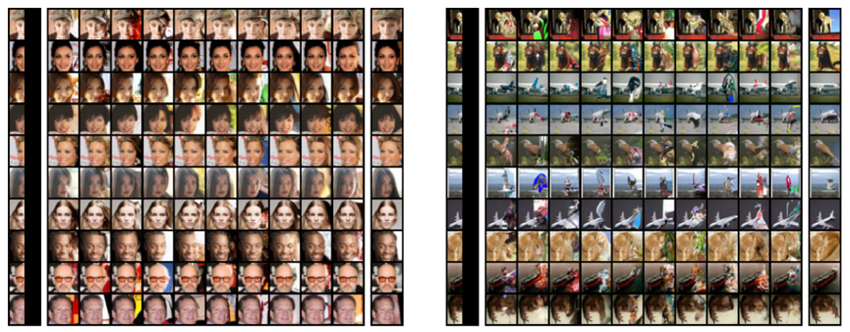
5.3. Image inpainting

Figure 6. 에서, NCSN 이 일반적이고 의미론적인 이미지의 표현 (representation) 을 학습해 image inpainting 을 가능하게 함을 보인다. PixelCNN 과 같은 이전 모델들의 경우, raster scan 을 따라서만 이미지를 색칠할 수 있다. 이와 달리, NCSN은 annealed Langevin dynamics 에 약간의 변형을 가하면 임의의 모양으로 지워진 (occluded) 이미지를 처리할 수 있다.

Figure 6. Image inpainting using NSCN (a) CelebA (b) CIFAR-10.
각 dataset 에 대한 이미지 중 가장 오른쪽 열이 원본 이미지를 나타낸다.
Source : Song & Ermon. (2019)

Algorithm for image inpainting.
Source : Song & Ermon. (2019)

Reference

[1] Yang Song and Stefano Ermon. Generative Modeling by Estimating Gradients of the Data Distribution. arXiv:1907.05600, 2019.