Adaboost

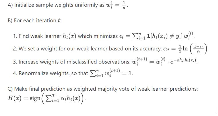
Adaptive + Boosting

Boosting : Reduce the Bias

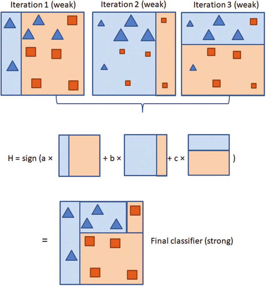
• 이전에 잘못 분류된 기록에 보다 집중하여 훈련 데이터의 분포를 적응적으로 변경하는 반복적인 절차
• Parallel(병렬) 작업이 아니라 Sequential(순차적) 과정

Strong Classifier : 개별 약분류기들에 가중치를 적용 및 조합하여 얻을 수 있음

Weak Classifier : 약분류기

장점

과적합이 덜합니다
적은 매개변수 조정
편향과 분산을 줄이는 데 도움이 됩니다
이 방법을 사용하면 약한 분류기의 정확도를 향상시킬 수 있습니다
사용하기 편함

단점

품질 데이터 세트가 필요합니다
이상치 및 소음에 매우 민감함
XGBoost보다 느린 속도
하이퍼파라미터 최적화는 훨씬 더 어렵습니다

Implementation

Creating a dataframe

First we will be creating a dataframe for whic we have to perform classification

df = pd.DataFrame()
df['feature1'] = [9,9,7,6,6,5,4,3,2,1]
df['feature2'] = [2,9,8,5,9,1,8,6,3,5]
df['target'] =[-1,-1,1,-1,1,-1,1,-1,1,1]
df['w'] = 1/df.shape[0]
df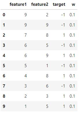

Separate the features and target variable

#features and target values
X = df.iloc[:,0:2].values
y = df.iloc[:,2].values

Plot the points in 2D Space

from typing import Optional
import numpy as np
import matplotlib.pyplot as plt
import matplotlib as mpl
#visualizing our datapoints
def plot_adaboost(X: np.ndarray,
                  y: np.ndarray,
                  clf=None,
                  sample_weights: Optional[np.ndarray] = None,
                  annotate: bool = False,
                  ax: Optional[mpl.axes.Axes] = None) -> None:
    assert set(y) == {-1, 1}, 'Expecting response labels to be ±1'
    if not ax:
        fig, ax = plt.subplots(figsize=(5, 5), dpi=100)
        fig.set_facecolor('white')
    pad = 1
    x_min, x_max = X[:, 0].min() - pad, X[:, 0].max() + pad
    y_min, y_max = X[:, 1].min() - pad, X[:, 1].max() + pad
    if sample_weights is not None:
        sizes = np.array(sample_weights) * X.shape[0] * 100
    else:
        sizes = np.ones(shape=X.shape[0]) * 100
    X_pos = X[y == 1]
    sizes_pos = sizes[y == 1]
    ax.scatter(*X_pos.T, s=sizes_pos, marker='+', color='green')
    X_neg = X[y == -1]
    sizes_neg = sizes[y == -1]
    ax.scatter(*X_neg.T, s=sizes_neg, marker='.', c='purple')
    if clf:
        plot_step = 0.01
        xx, yy = np.meshgrid(np.arange(x_min, x_max, plot_step),
                             np.arange(y_min, y_max, plot_step))
        Z = clf.predict(np.c_[xx.ravel(), yy.ravel()])
        Z = Z.reshape(xx.shape)
     
        if list(np.unique(Z)) == [1]:
            fill_colors = ['g']
        else:
            fill_colors = ['purple', 'g']
        ax.contourf(xx, yy, Z, colors=fill_colors, alpha=0.2)
    if annotate:
        for i, (x, y) in enumerate(X):
            offset = 0.05
            ax.annotate(f'$x_{i + 1}$', (x + offset, y - offset))
    ax.set_xlim(x_min+0.5, x_max-0.5)
    ax.set_ylim(y_min+0.5, y_max-0.5)
    ax.set_xlabel('$x_1$')
    ax.set_ylabel('$x_2$')
plot_adaboost(X, y)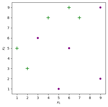

Create a class AdaBoost with variables like stumps, errors etc.

class AdaBoost:
    def __init__(self):
        self.stumps = None
        self.stump_weights = None
        self.errors = None
        self.sample_weights = None

    def _check_X_y(self, X, y):
        assert set(y) == {-1, 1}, 'Response variable must be ±1'
        return X, y
        

여기서 우리는 최대 깊이 = 1인 Decision tree를 다음과 같이 사용했습니다
우리의 기본 분류기입니다. Adaboost는 이 약한 학습자에게 훈련 데이터의 다른 분포를 제공할 때마다 반복적으로 이 학습자를 호출합니다. 우리가 호출할 때마다 약한 분류기를 생성하고 이 모든 분류기를 하나의 분류기로 결합하여 더 나은 성능을 제공합니다.

from sklearn.tree import DecisionTreeClassifier
def fit(self, X: np.ndarray, y: np.ndarray, iters: int):
    X, y = self._check_X_y(X, y)
    n = X.shape[0]
    self.sample_weights = np.zeros(shape=(iters, n))
    self.stumps = np.zeros(shape=iters, dtype=object)
    self.stump_weights = np.zeros(shape=iters)
    self.errors = np.zeros(shape=iters)
    self.sample_weights[0] = np.ones(shape=n) / n
    for t in range(iters):
        curr_sample_weights = self.sample_weights[t]
        stump = DecisionTreeClassifier(max_depth=1, max_leaf_nodes=2)
        stump = stump.fit(X, y, sample_weight=curr_sample_weights)
        stump_pred = stump.predict(X)
        err = curr_sample_weights[(stump_pred != y)].sum()# / n
        stump_weight = np.log((1 - err) / err) / 2
        new_sample_weights = (curr_sample_weights * np.exp(-stump_weight * y * stump_pred))
        new_sample_weights /= new_sample_weights.sum()
        if t+1 < iters:
            self.sample_weights[t+1] = new_sample_weights
        self.stumps[t] = stump
        self.stump_weights[t] = stump_weight
        self.errors[t] = err
    return self
def predict(self, X):
    stump_preds = np.array([stump.predict(X) for stump in self.stumps])
    return np.sign(np.dot(self.stump_weights, stump_preds))
AdaBoost.fit = fit
AdaBoost.predict = predict
clf = AdaBoost().fit(X, y, iters=10)
plot_adaboost(X, y, clf)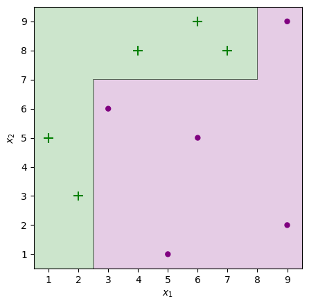

Visualizing our learner step by step

여기서 왼쪽 열은 선택된 약한 학습자를 나타내고 오른쪽 열은 각 반복에서 지금까지 얻은 누적 강한 학습자를 나타냅니다. Adaboost 분류기에 따르면 이전 반복에서 잘못 분류된 점은 이제 더 가중치가 부여되어 다음 반복에서 더 크게 나타납니다.

def truncate_adaboost(clf, t: int):
    assert t > 0, 't must be a positive integer'
    from copy import deepcopy
    new_clf = deepcopy(clf)
    new_clf.stumps = clf.stumps[:t]
    new_clf.stump_weights = clf.stump_weights[:t]
    return new_clf

def plot_staged_adaboost(X, y, clf, iters=10):
    fig, axes = plt.subplots(figsize=(8, iters*3),
                             nrows=iters,
                             ncols=2,
                             sharex=True,
                             dpi=100)
    fig.set_facecolor('white')
    _ = fig.suptitle('Decision boundaries by iteration')
    for i in range(iters):
        ax1, ax2 = axes[i]
        _ = ax1.set_title(f'Weak learner at t={i + 1}')
        plot_adaboost(X, y, clf.stumps[i],
                      sample_weights=clf.sample_weights[i],
                      annotate=False, ax=ax1)
        trunc_clf = truncate_adaboost(clf, t=i + 1)
        _ = ax2.set_title(f'Strong learner at t={i + 1}')
        plot_adaboost(X, y, trunc_clf,
                      sample_weights=clf.sample_weights[i],
                      annotate=False, ax=ax2)
    plt.tight_layout()
    plt.subplots_adjust(top=0.95)
    plt.show()
clf = AdaBoost().fit(X, y, iters=10)
plot_staged_adaboost(X, y, clf)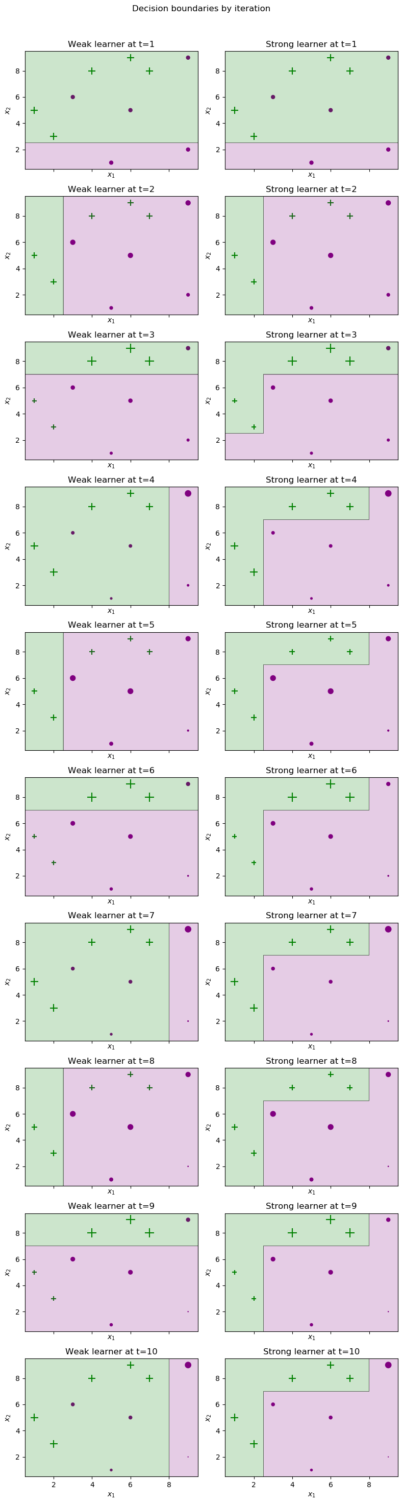

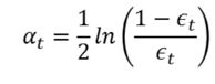
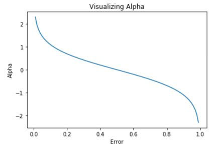
Plot for error rate is as follows-

The error rate is:

Comparison with sklearn’s inbuilt adaboost classifier

사용된 n_estimator는 1, 5, 10개의 트리로 성능 차이를 인지하고 모델을 부스팅하는 작업을 이해하는 데 도움이 됩니다.
Split the dataset into 70:30

from sklearn.model_selection import train_test_split
X_train, X_test, y_train, y_test = train_test_split(X, y, test_size=0.3)

Adaboost classifier with n_estimators=1

from sklearn.ensemble import AdaBoostClassifier
from sklearn import metrics
abc = AdaBoostClassifier(n_estimators=1,learning_rate=1)
model = abc.fit(X_train, y_train)
y_pred = model.predict(X_test)
plot_adaboost(X, y, model)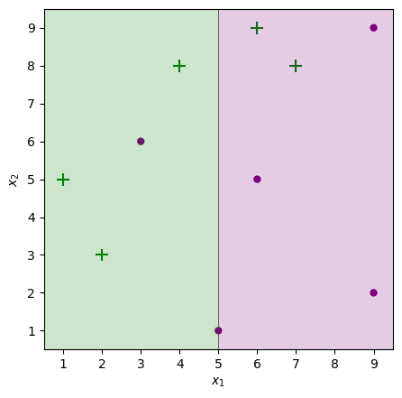

Adaboost classifier with n_estimators=5

from sklearn.ensemble import AdaBoostClassifier
from sklearn import metrics
abc = AdaBoostClassifier(n_estimators=5,learning_rate=1)
model = abc.fit(X_train, y_train)
y_pred = model.predict(X_test)
plot_adaboost(X, y, model)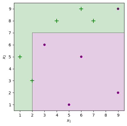

Adaboost classifier with n_estimators=10

from sklearn.ensemble import AdaBoostClassifier
from sklearn import metrics
abc = AdaBoostClassifier(n_estimators=10,learning_rate=1)
model = abc.fit(X_train, y_train)
y_pred = model.predict(X_test)
plot_adaboost(X, y, model)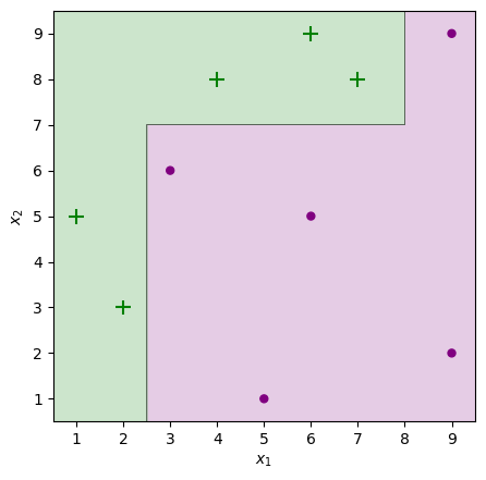

결론

의사결정 트리는 기본 분류기로 사용됩니다
여전히 약한 분류기를 사용했지만 모든 인스턴스가 올바르게 분류됩니다.
분류기의 주요 원리는 잘못 분류된 데이터 포인트의 가중치를 높이고 올바르게 분류된 포인트의 가중치 값을 줄이는 것입니다. 이렇게 분류기에서 가중치를 업데이트하면 다음 반복의 약한 학습자가 의미 있는 결정 경계를 가질 수 있습니다.
트리가 증가하면 모델은 더 나은 정확한 분류를 제공합니다.