Geometry Processing with Neural Fields

https://proceedings.neurips.cc/paper/2021/hash/bd686fd640be98efaae0091fa301e613-Abstract.html

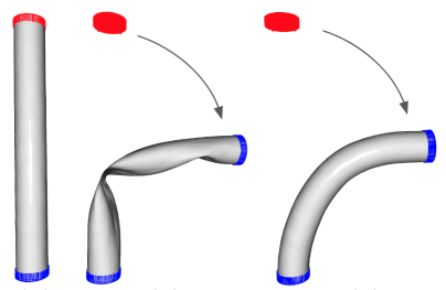
동기: NeRF로 학습된 object의 shape을 원하는데로 deform할 수 있을까?
NeRF-Editing: Geometry Editing of Neural Radiance Fields 같은 경우는 메쉬로 변환하고 ARAP으로 변형한다음 결과를 다시 NeRF에 적용했다. 변형에 걸리는 시간은 ARAP이 더 빠르겠지만 어떻게 meshing 하느냐에 따라 결과가 달라질 것이다. 이 논문은 아예 새로운 network를 하나 학습시켜 계산량이 많은데, 문제 푸는 방식은 더 정석적이다.

Smoothing, sharpening은 optimization 통해서 새 파라미터를 훈련시켜서 만드는데 각 항은, 원본 유지, normal 유지, curvature 변형으로 이루어져있다.

Deformation을 위해서는 먼저 zero isosurface 위에 있는 점들을 sampling 한다. 저자들은 Langevin dynamics를 이용한 $\mathbf{x}_{t+1}=\tilde{\mathbf{x}}_t-F(\tilde{\mathbf{x}}_t)n_F(\tilde{\mathbf{x}}_t)$, $\tilde{\mathbf{x}}_t\sim \mathcal{N} (\mathbf{x}_t, \sigma \mathbf{I})$ 식을 따라 sampling 하였다. 이 때, $\mathbf{x}_0$은 [-1, 1]에서 sampling됨. 이 때, point들이 curvature가 큰 구간에 집중되는 현상을 막기 위해서 첫 sampling때 surface에서 너무 먼 점들은 (-1,1로 normalize된 공간에서 거리가 0.1 이상) reject하는 식으로 꽤 균일하게 얻어낼 수 있었다고 한다. 이게 첫 $\mathbf{x}_0$은 그냥 [-1, 1]에서 sampling하고 그 주변 점들을 Langevin dynamics를 이용해 수차례 반복해서 얻고, 다시 새 $\mathbf{x}_0$을 찾아서 반복하는 방식인 것 같다.

Deformation field는 neural network $D_\theta$에 의해 정의되는 neural field이다. 이 때, 원 공간과 deform 공간의 one-to-one correspondence를 보장하기 위해 $D_\theta$를 invertible하게 설계한다. NeRF 등에서 말하듯 MLP를 이용해서 복잡한 prediction을 하려면 $\sin(ax+b)$같은 periodic function을 사용하는 것이 좋은데 (Fourier features let networks learn high frequency functions in low dimensional domains 참조), Invertible residual networks에 따르면 $f(x)=x+g(x)$가 invertible하기 위한 충분 조건은 $g$의 Lipschitz constant가 1보다 작아야한다. 따라서 periodic function을 normalize한 $|a|^{-1}\sin(ax+b)$을 사용할 것이고, 구체적으로 positional encoding은

이 되고, 각 residual block은

이다. 저자들이 ablation study 해본 결과, deformation field가 invertible하지 않은 경우 topology가 깨지고, positional encoding하지 않는 경우 복잡한 변형을 예측하지 못했다.

이제 우리는 deformed 공간의 $\mathbf{x}$를 입력으로 받아 input 공간의 $\mathbf{y}$를 출력하는 $D_\theta$를 얻었다. $D_\theta$를 훈련시키기 위한 loss는 stretching과 bending을 줄일 수 있도록 설계한다. 먼저 stretching은 surface의 tangent vector의 길이 변화로(이는 다시 tangent vector의 dot-product로) 측정될 수 있다. 먼저 tanget vector를 구해야하는데, $\mathbf{n}_{G_\theta}(\mathbf{x})$를 $\mathbf x$에서의 surface normal이라고 하면 tangent space에 대한 projection matrix는 $\mathbf{P}_{G_{\theta}}(\mathbf{x})=\mathbf{I}-\mathbf{n}_{G_\theta}(\mathbf{x})\mathbf{n}_{G_\theta}(\mathbf{x})^{T}$이다. 그렇다면 임의의 vector $\mathbf{v}$에 대해 tanget vector는 $\mathbf{P}_{G_{\theta}}(\mathbf{x})\mathbf{v}$이다. (근데 임의의 $\mathbf{v}$는 어떻게 구한다는거지?) 이제 tangent dot-product의 변화를 계산해보자. $\mathbf{t}_i$, $\mathbf{t}_j$를 deformed 공간의 점 $\mathbf{x}$에서의 임의의 두 tangent vector라고 하자. $D_\theta$에 의해 transform 하면 $\mathbf{t}'=\mathbf{J}_{D_\theta}(\mathbf{x})\mathbf{t}$ 일 것이다 (Jacobian과 tangent space 관계 참조).

이 차이를 minimize하기 위해서는 앞뒤의 $\mathbf{v}$를 drop하고 가운데만 minimize 해도 된다.

이다.

Bending은 surface의 curvature의 변화로 볼 수 있다. 이는 surface normal direction을 따른 tangent dot product의 변화로 측정될 수 있으니, curvature를 directional derivative 또는 Hessian을 이용해 구할 수 있다.

이 때, $t$는 $\mathbf{x}+t\mathbf{n}(\mathbf{x})$에 의해 normal 방향 성분이다. 그래서 curvature의 변화는

stretching loss와 마찬가지로

훈련 과정에서 $D_\theta$가 valid한 SDF일 것이라 보장할 수 없다. 따라서 다음의 변형을 이용해 $\mathbf{x}$대신 $\mathbf{y}$를 sample해서 loss를 계산한다.

마지막으로 user input에 대한 constaint

최종 loss는 위 세 loss들의 weighted sum이다.