NeRF: Representing Scenes as Neural Radiance Fields for View Synthesis (Original paper)
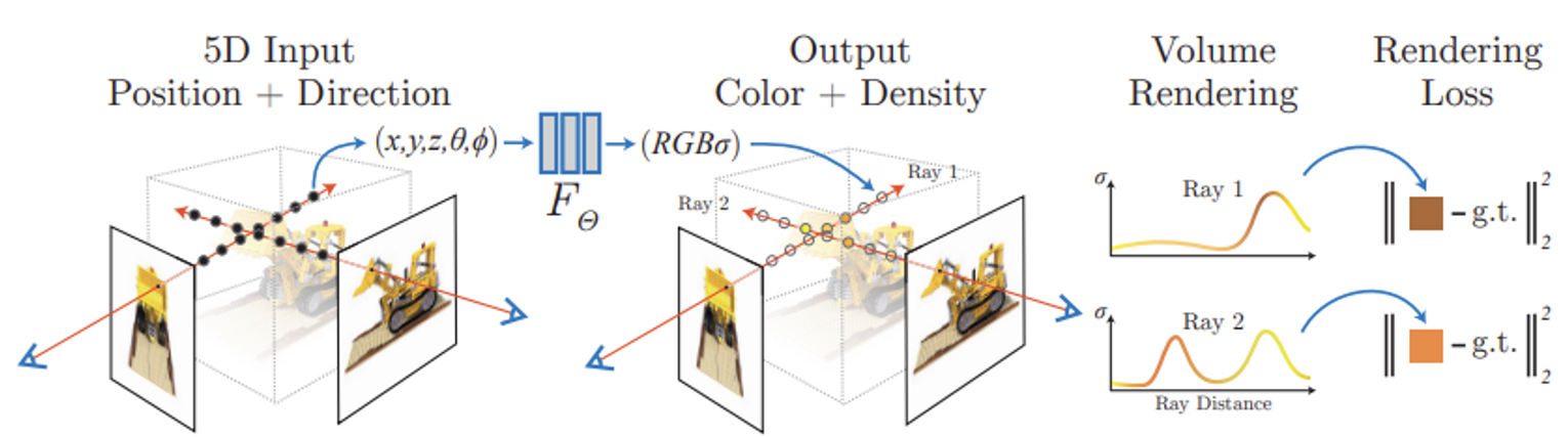
FΘ:(x,d)→(c,σ)
Volume density σ는 3D location x만 가지고 결정하고(어느 방향에서 바라보든 모양은 같다.) emitted color c는 x와 viewing direcion d를 함께 이용해 결정한다.
Camera position o로부터 camera ray r(t)=o+td에 대하여 color C(r)을 계산한다.
C(r)=∫tntfT(t)σ(r(t))c(r(t),d)dtwhereT(t)=exp(−∫tntσ(r(s))ds)
이 때, tn과 tf는 각각 ray의 near, far bound이며, T(t)는 ray가 tn에서 t까지 도달할 확률을 의미한다. 즉, 전체적인 의미는, 이전에 다른 particle에 부딪히지 않았던 ray가, particle에 부딪혔을 때 그 색깔을 나타낸다.
실제로는 integral을 계산하기 어려워서 quadrature (구적법)을 사용한다. 모델이 항상 비슷한 위치에서 query 되는 것을 방지하기 위해 다음과 같이 random하게 sampling 한다. 우선 [tn,tf]를 N개로 균등하게 나누고 각 bin에서 uniform하게 대표값을 뽑는다. 즉,
ti∼U[tn+Ni−1(tf−tn),tn+Ni(tf−tn)]
이다. 그럼 위의 적분 식이 다음과 같이 discrete 하게 표현될 수 있다.
C^(r)=i=1∑NTi(1−exp(−σiδi))ciwhereTi=exp(−j=1∑i−1σjδj)
이 때, δi=ti+1−ti은 이웃한 sample간의 거리이다. αi=1−exp(−σiδi)는 일반적인 alpha 값으로 볼 수 있다. Implementation detail 단락을 보면 σ은 activation을 거치지 않는 것으로 나오는데, 그 값을 0~1 사이로 강제하려고 이렇게 변환한 것 같기도하다.
저자들이 과거에 썼던 논문 중에 삼각함수를 이용해서 입력을 중복해서 (정확히는 다른 주파수 커널로 맵핑해서) 넣어주면 high frequency 성능이 향상된다는 내용이 있다. 이를 positional encoding이라고 부르고 (transformer의 positional encoding과는 다르다) NeRF에도 적용했다.
γ(p)=(sin(20πp),cos(20πp),⋯,sin(2L−1πp),cos(2L−1πp))
한 개의 모델만 가지고는 성능이 만족스럽지 못해서, fine한 모델을 하나 더 도입한다. 차이는 fine한 모델을 coarse한 모델이 sampling 한 결과를 가지고 더 나은 sampling 한 point만을 가지고 학습된다는 것이다. 두 모델을 동시에 학습하며 loss는 다음과 같다.
L=r∈R∑[∣∣C^c(r)−C(r)∣∣22+∣∣C^f(r)−C(r)∣∣22]
사소한 Implementation detail - 5번째 layer에 x를 feature vector에 concat해서 다시 한 번 넣어줌. 훈련 시 σ를 ReLU에 통과하기 전에 Gaussian noise n∼N(0,1)을 더해줌.
한계: 각 모델마다 한 개의 scene 밖에 학습하지 못함. 매 학습이 독립적이라 기존 학습한 모델로부터 공통된 정보를 가져올 수 없음. 정제된 데이터에 대해서만 잘 작동 (multiview consistent한 constraint이 강함)
NeRF in the Wild: Neural Radiance Fields for Unconstrained Photo Collections
동기: NeRF는 view consistency가 강력하게 지켜진 정제된 이미지에서는 잘 동작하지만 in the wild 이미지에는 잘 동작하지 않는다.
In the wild 이미지에는 original NeRF에서 가정했던 consistency가 1) Photometric variation (즉, color c가 달라짐), 2) transient objects (즉, volume density σ가 달라짐) 관점에서 달라진다.
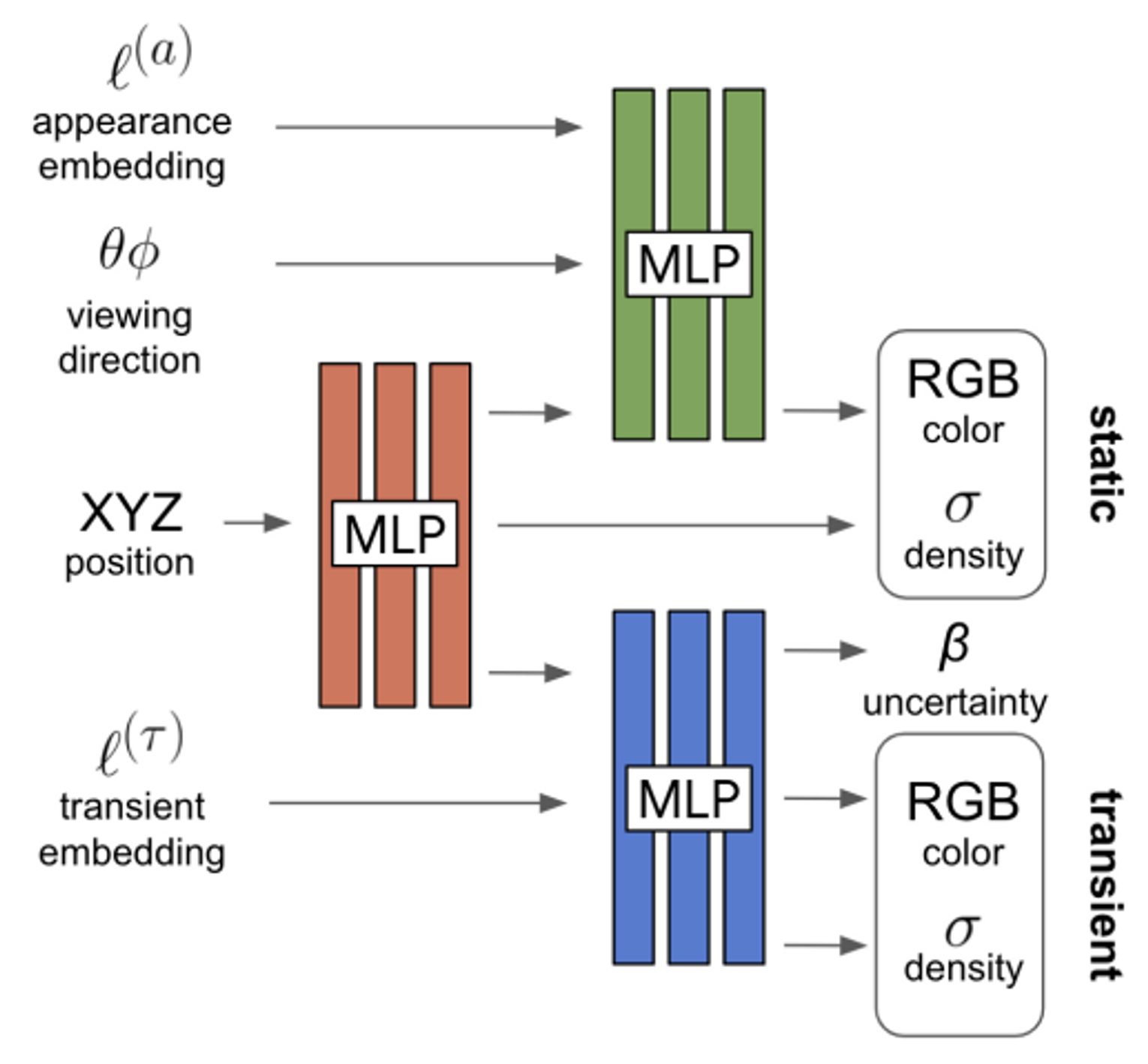
color는 이미지 Ii에 따라 바뀌어야 한다. 이를 위해 GLO를 이용하여 얻은 이미지 Ii에 대한 appearance embedding vector li(a)를 모델에 입력해준다.
Transient object를 표현하기 위해 기존의 NeRF모델을 static한 부분을 나타내는 것으로 놔두고, transient한 부분을 표현하기 위한 MLP를 하나 추가한다. static한 color, density를 각각 c, σ라 하고, transient한 color, density를 각각 c(τ), σ(τ)라 하면,
C^i(r)=k=1∑KTi(tk)(α(σ(tk)δk)ci(tk)+α(σi(τ)(tk)δk)ci(τ)(tk))whereTi(tk)=exp⎝⎜⎛−k′=1∑k−1(σ(tk′)+σi(τ)(tk′))δk′⎠⎟⎞
Uncertainty를 학습하기 위해 color를 Ci(r)∼N(C^i(r),βi(r)2)로 모델한다.
위 그림에 적갈색을 MLP1, 녹색을 MLP2, 청색을 MLP3이라 하면
[σ(t),z(t)]=MLPθ1(γx(r(t)))ci(t)=MLPθ2(z(t),γd(d),li(a))[σi(τ)(t),ci(τ)(t),βi(t)]=MLPθ3(z(t),li(τ))
더불어, transient한 MLP는 Bayesian learning을 통해 observed color의 uncertainty를 출력한다. (Bayesian deep learning은 링크 글 참조)
Loss는
Li(r)=2βi(r)2∣∣Ci(r)−C^i(r)∣∣22+2logβi(r)2+Kλuk=1∑Kσi(τ)(tk)
이 식을 보면 앞에 두 term은 Ci(r)이 N(C^i(r),βi(r)2)을 따를 때 negative log likelihood이다. 마지막 term은 모델이 모든 부분이 transient하다고 결론내리는 것을 방지하기위한 regularizer다. 최종적으로는 위의 loss로 fine 모델을 학습하고 original NeRF와 같이 l2 norm만 가지고 학습되는 coarse 모델이 하나 더 있다.
동기: 사진마다 deform이 있을 수 있다면 어떻게 해야할까?
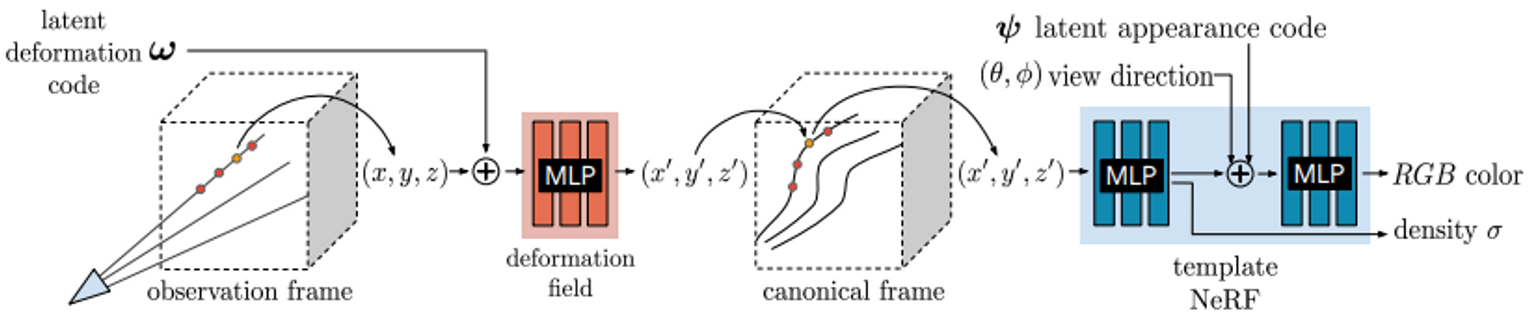
Observation 공간과 canonical 공간 사이를 mapping하는 MLP를 추가함.
GRAF: Generative Radiance Fields for 3D-Aware Image Synthesis
동기: NeRF를 바탕으로 3D generative model을 만들어보자
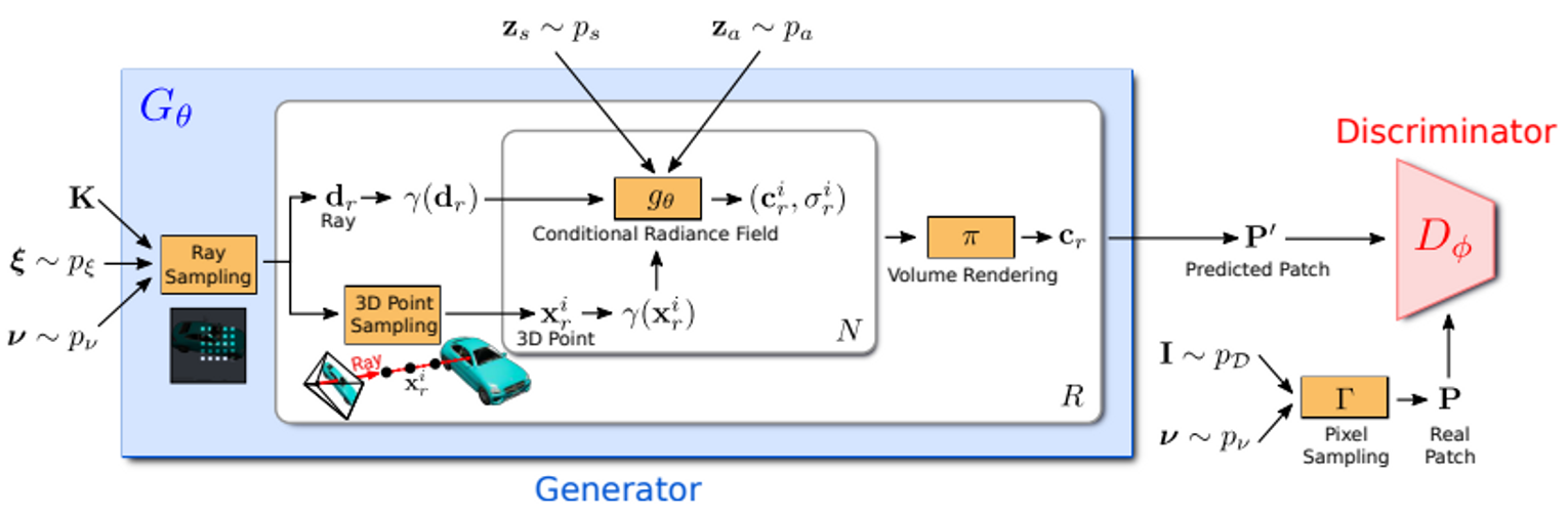
전체적인 구조. 여기서 Conditional Radiance Field gθ와 Discriminator Dϕ만 딥러닝 모델이다.
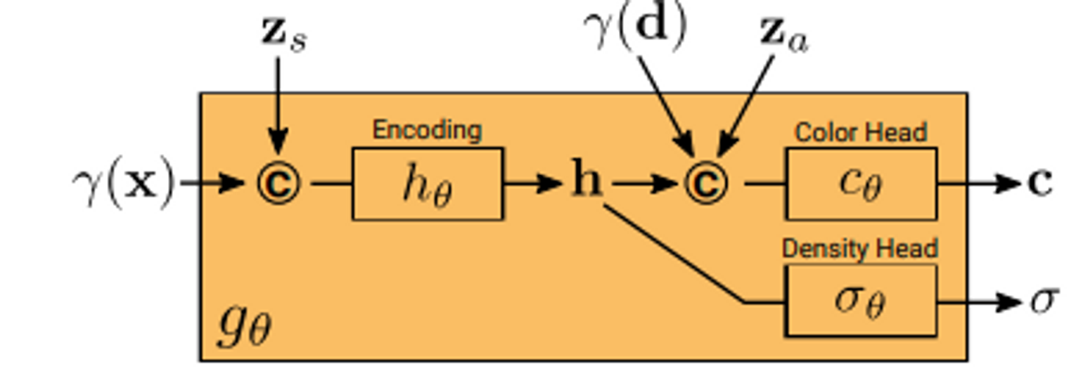
Conditional Radiance Field의 생김새이다. GAN의 역할을 하기 위해 shape code zs와 appearance code za를 추가로 입력받는 것을 볼 수 있다.
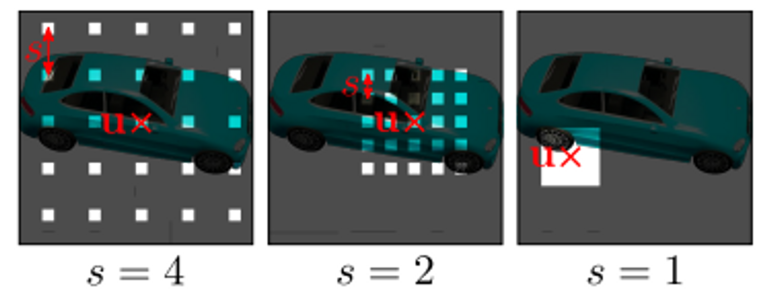
Discriminator는 generator에서 생성된 patch와 학습 이미지에서 생성된 patch를 가지고 학습되는데, 항상 K x K 크기를 random 한 scale을 가지고 sampling해서 학습한다.
pixelNeRF: Neural Radiance Fields from One or Few Images
동기: NeRF는 각각의 scene을 학습하기 위해 많은 수 (original paper에서는 scene 당 100장)의 사진을 필요로 한다. 어떻게 하면 prior 정보를 이용해 필요한 사진의 수를 줄일 수 있을까?
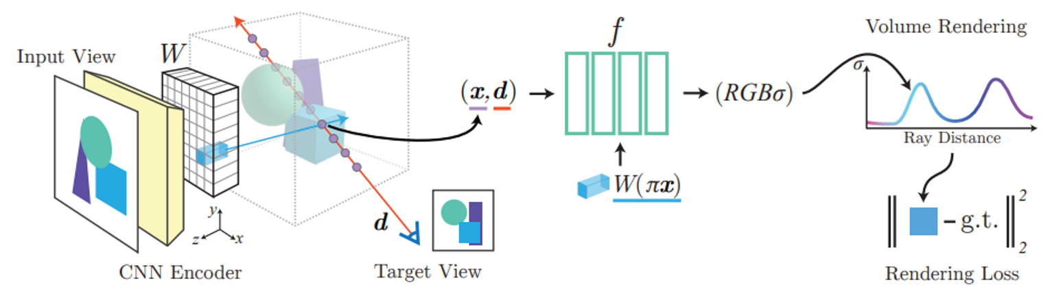
Image로 NeRF를 condition하자 (입력에 image embedding을 같이 넣어주자). Fully convolutional image encoder E를 도입한다. 입력 이미지 I에 대한 feature volume은 W=E(I)이다. 3D position을 이미지 plane에 project 하는 함수를 π(⋅)라 하면, 3D position x의 feature vector는 W(π(x))이 된다. 이걸 NeRF에 같이 넣어준다.
f(γ(x),d;W(π(x))=(σ,c)
위의 경우는 훈련 시, 또는 이미지 한 장에 대해 추론할 때 적용된다. 만약에 추론 시 이미지 여러장을 입력해 결과를 개선하고 싶다면, NeRF f를 initial layer들 f1과 final layer들 f2로 나누어서, 여러 이미지에 대한 f1의 출력을 average pooling하여 f2에 입력한다.
한계: average pooling은 너무 naive하다. 분명히 가중치를 주거나 더 잘 합치는 방법이 있을 것.
NeuS: Learning Neural Implicit Surfaces by Volume Rendering for Multi-view Reconstruction
동기: 기존의 neural surface rendering은 surface의 급격한 depth 변화에 알맞지 않고, NeRF를 비롯한 volume rendering은 surface의 품질이 떨어진다. 두 방법론의 장점만 취해보자.
SDF를 volume으로 변환하기 위해 ϕs(x)=se−sx/(1+e−sx)2 를 도입했다(sigmoid의 derivative다). SDF를 변환한 ϕs(f(x))를 S-density라 부르자.
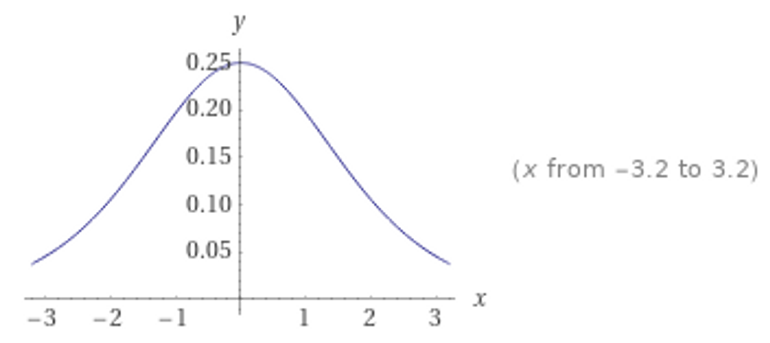
ϕs(x) 그래프
Ray의 식이 p(t)=o+tv 일 때, volume rendering의 식을 아래처럼 표현하자.
C(o,v)=∫0+∞w(t)c(p(t),v)dt
w(t)는 weight인데 original NeRF에서는 w(t)=T(t)σ(r(t)) 였다. 이 weight를 새로 제시하는 것이 이 논문의 목적이다. weight는 1) unbiased: surface에서 local maximum value를 가져야하며 2) occlusion-aware: S-density가 같은 두 point가 있으면 view point에 가까운 point가 최종 color에 영향을 더 많이 미쳐야한다. original NeRF의 weight은 occlusion-aware하지만 biased이다. 그래서 아래의 함수들을 사용하는데, 어떻게 나온 것인지는 논문의 유도를 참조하자.
w(t)=T(t)ρ(t)T(t)=exp(−∫0tρ(u)du)ρ(t)=max(Φs(f(p(t)))−dtdΦs(f(p(t))),0)
Neural Sparse Voxel Fields
동기: NeRF에서 고해상도 이미지를 얻기 위해서는 ray marching의 계산 복잡도가 높음. 적은 계산 복잡도로 얻는 결과는 blurry함.
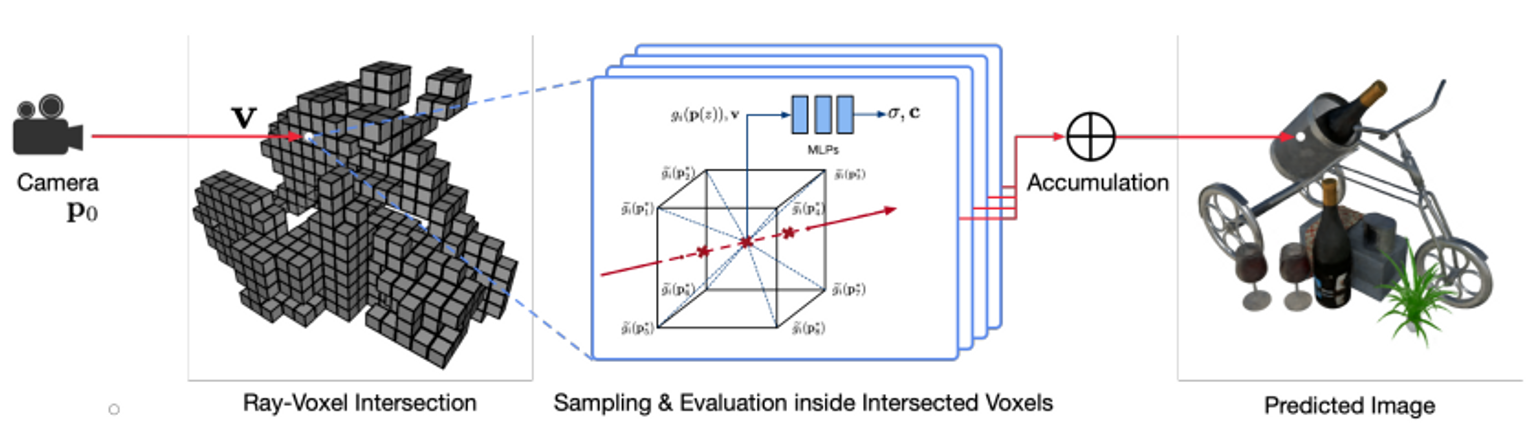
Scene이 sparse (bounding) voxels V={V1,…,VK}로 구성되어 있다고 했을 때, voxel i에서 scene은 voxel-bounded implicit function Fθi로 나타내어질 수 있다.
Fθi:(gi(p),v)→(c,σ),∀p∈Vi
gi(p)=ζ(χ(gi~(p1∗),…,gi~(p8∗)))
χ는 trilinear interpolation, ζ는 post processing (여기서는 구체적으로 positional encoding).gi(p)=ζ(p) 면 NeRF와 같다.
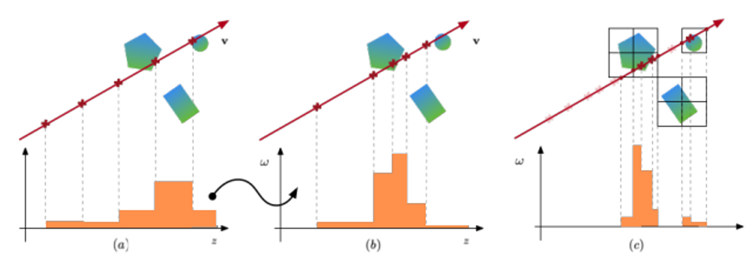
Volume rendering은 1) AABB tree를 이용한 ray-voxel intersection, 2) Voxel 안에서 ray-marching, 총 두 단계로 이루어진다.
NeRF-Editing: Geometry Editing of Neural Radiance Fields
동기: NeRF로 학습된 object의 shape을 원하는데로 deform할 수 있을까?
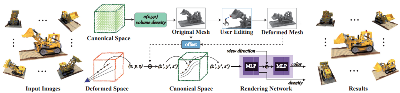
메쉬로 변환하여 editing (As-rigid-as possible 이용)하고 이를 바탕으로 deformed space와 canonical space의 관계를 정의함. 이 때, 메쉬를 NeuS처럼 SDF로 정의하며, deformed space를 정의할 때 약간의 테크닉이 들어감.