지금까지 우리는 k-NN classification, k-NN regression, linear regression, 그리고 polynomial regression 에 대해 알아보았다. 이번에는 multiple (multinomial) regression 과 feature engineering 을 공부해보자.
Contents
- Multiple regression
- Feature engineering
- Data preparation with Pandas
- Creating PolynomialFeatures with sklearn
- Training LinearRegression()
1. Multiple regression
Multiple regression 은 polynomial regression 과 헷갈릴 수 있지만 다음과 같은 이유로 다른 개념이다.
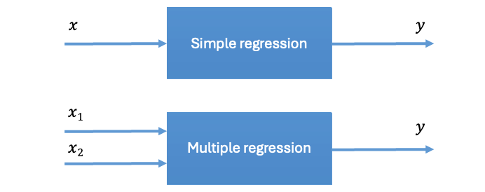
- Polynomial regression is about improving our model’s closeness to the data by increasing the order of the relationships between the factors and the response variables.
Ex)
- Multiple regression we’re interested in the impact of not only one, but many different factors, on the response variable. This is usually representative of real world problems.
Ex)
따라서 multiple regression 에서 특성의 개수가 증가할수록 우리의 모델은 점점 고차원의 hyperplane 의 방정식을 학습하게 된다. 하지만 그래프로 나타내는 것에도 한계가 존재하게 된다.
2. Feature engineering
A machine learning technique that leverages data to create new variables that aren't in the training set. The goal is to simplify and speed up data transformations while also enhancing model accuracy.
Machine learning 에서 feature engineering 은 매우 중요한 단계 중 하나이다. 간단히 말하자면 feature engineering 은 새로운 특성을 추가하거나 변경 및 조합하는 등의 과정이다.
- 특히 machine learning 알고리즘들이 feature engineering 에 영향을 많이 받는 반면, deep learning 모델들은 feature engineering 이 요구되지 않거나 비교적 영향이 덜하다.
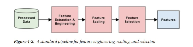
따라서, multiple regression 을 구현하기 위해 우리는 sklearn 의 feature engineering tool 을 이용해 샘플들을 preprocessing 해주어야 한다.
3. Data preparation with Pandas
우선 전처리를 해주기에 앞서 Pandas 로 데이터를 준비해보자. Pandas 는 data manipulation 및 analysis 를 위한 Python 의 핵심 software library 중 하나이다. 참고로 Pandas 를 비롯한 다른 핵심 패키지들에는 SciPy, Numpy, sklearn, matplotlib 등이 있다.
DataFrame (df) is a 2-dimensional labeled data structure with columns of potentially different types. It is generally the most commonly used pandas object.
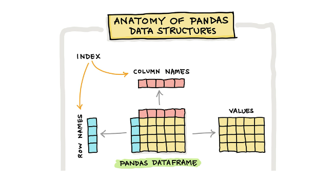
Pandas 의 주요 data structure 는 Dataframe 라고 하는 것이다. 이는 2차원의 배열로 spreadsheet 나 SQL table 과 비슷하다고 보면 된다. 특히 Numpy 의 ndarray 와는 다르게 mutable 하여 여러 종류의 데이터를 담을 수 있는 장점이 있다. 또한 Pandas 는 간단히 통계치를 만들거나, 인터넷에서 데이터를 불러와 manipulate 및 visualize 할 수 있는 기능이 풍부하기에 널리 쓰여왔다.
이번에 우리는 broccoli 의 길이뿐만 아니라 높이와 두께를 참고해 무게를 예측해 볼 것이다.
1) pd.read_csv() 로 데이터를 불러와 to_Numpy() 를 통해 Numpy array 로 변환
- 참고로 csv file 은 comma 로 나눠져있는 단순한 text file 이다.
import pandas as pd

df = pd.read_csv('https://bit.ly/broccoli_csv')
broccoli_full = df.to_numpy()
2) train_test_split 적용
from sklearn.model_selection import train_test_split

train_input, test_input, train_target, test_target = train_test_split(broccoli_full, broccoli_weight)
4. Creating PolynomialFeatures with sklearn
앞서 말했듯이 sklearn 에서는 PolynomialFeatures 라고 하는 class 를 제공한다. 해당 class 는 자동으로 절편을 위한 "bias" 로 특성 "1" 을 생성하며, 이는 배열끼리의 곱셈 연산 등에 유용하게 쓰인다. 하지만 linear regression 은 이를 무시하기 때문에 있어도 되고 없어도 되는 값이다. 굳이 "1" 의 특성을 만들지 않기 위해서는 아래와 같이 bias 를 False 로 지정해주면 된다.
Functions of the PolynomialFeatures class squares or multiplies the existing features to create new features.
from sklearn.preprocessing import PolynomialFeatures

poly = PolynomialFeatures(include_bias=False)
poly.fit(train_input)
train_poly = poly.transform(train_input)
test_poly = poly.transform(test_input)
PolynomialFeatures 를 생성하기 위해 우리는 먼저 fit 을 통하여 존재하는 특성들을 학습 후, transform 을 적용해 곱셈이나 제곱의 연산을 통해 새로운 특성들을 만들어 준 것이다. 참고로 fit 과 transform 을 한번에 처리해주는 fit_transform() method 도 존재한다.
또한 PolynomialFeatures class 의 degree = 2 가 default 이므로 평소 제곱까지만 연산하지만, 이 값을 증가시킨다면 더 높은 거듭제곱 특성들을 얻을 수 있다.
print(train_poly.shape) # (42,9)
print(poly.get_feature_names_out()) # ['x0' 'x1' 'x2' 'x0^2' 'x0 x1' 'x0 x2' 'x1^2' 'x1 x2' 'x2^2']
결과적으로 우리의 train_poly 는 기존 train_input 의 세 가지 특성에서 **9 가지의 특성**으로 늘어났음을 알 수 있다. 이와 관련한 연산을 더 자세히 알고싶다면 feature names 를 출력하는 함수를 이용하면 된다.
5. Training LinearRegression()
지금까지 feature engineering 을 통해 우리의 데이터 전처리를 완료하였다. 이후에는 지금까지 해왔던 것과 동일하게 linear regression model 을 훈련시킨 후 train 과 test set 에 대한 score 를 기반으로 성능을 확인해보자.
from sklearn.linear_model import LinearRegression

lr = LinearRegression()
lr.fit(train_poly, train_target)
print(lr.score(train_poly, train_target)) # 0.9896941207238812
print(lr.score(test_poly, test_target)) # 0.9827475645929417
아주 약간의 차이로 train set 에 대한 점수가 더 높은 것을 확인할 수 있다. 이는 분명 우리가 기존의 모델보다 더 많은 특성을 이용하여 예측했기에 훈련 세트에 잘 맞는 좀 더 복잡한 모델이 만들어졌기 때문일 것이다.
