import numpy as np
import pandas as pd
import seaborn as sns
import matplotlib.pyplot as plt
iris=pd.read_csv("C:/Users/pacif/kaggle/20240510 Iris/Iris.csv")iris.head(2)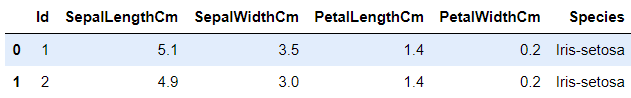
iris.info()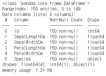
iris.drop('Id', axis=1, inplace=True)
#Id column을 제거하고 바로 dataframe에 적용하는 코드
#inplace=True가 dataframe에 적용하는 부분이다.
fig=iris[iris.Species=='Iris-setosa'].plot(kind='scatter', x='SepalLengthCm', y='SepalWidthCm', color='orange', label='Setosa')
iris[iris.Species=='Iris-versicolor'].plot(kind='scatter', x='SepalLengthCm', y='SepalWidthCm', color='blue', label='Setosa', ax=fig)
iris[iris.Species=='Iris-virginica'].plot(kind='scatter', x='SepalLengthCm', y='SepalWidthCm', color='green', label='Setosa', ax=fig)
fig.set_xlabel("Sepal Length")
fig.set_ylabel("Sepal Width")
fig.set_title("Sepal Length VS Width")
fig=plt.gcf()
fig.set_size_inches(10,6)
plt.show()
#sepal length와 width 사이의 관계를 보여주는 그래프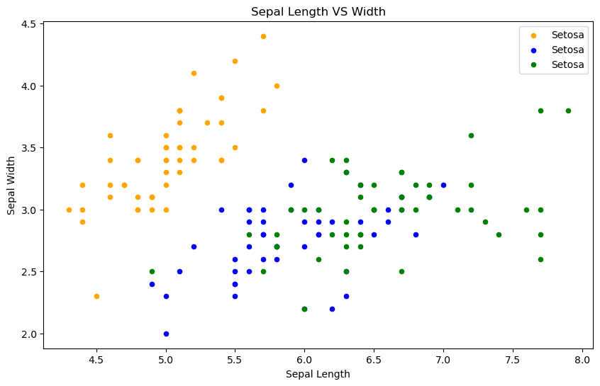
fig=iris[iris.Species=='Iris-setosa'].plot.scatter(x='PetalLengthCm', y='PetalWidthCm', color='orange', label='Setosa')
iris[iris.Species=='Iris-versicolor'].plot.scatter(x='PetalLengthCm', y='PetalWidthCm', color='blue', label='versicolor', ax=fig)
iris[iris.Species=='Iris-virginica'].plot.scatter(x='PetalLengthCm', y='PetalWidthCm', color='green', label='virginica', ax=fig)
fig.set_xlabel("Petal Length")
fig.set_ylabel("Petal Width")
fig.set_title("Petal Length VS Width")
fig=plt.gcf()
fig.set_size_inches(10,6)
plt.show()

#Petal 특성이 더 잘 분리되어있는 것을 알 수 있다.
#Sepal보다 Petal이 예측에 더 높은 정확도를 가져올 수 있을 것 같다.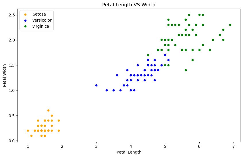
iris.hist(edgecolor='black', linewidth=1.2)
fig=plt.gcf()
fig.set_size_inches(12,6)
plt.show()
#iris dataset의 length와 width가 어떻게 분류되어있는지를 보자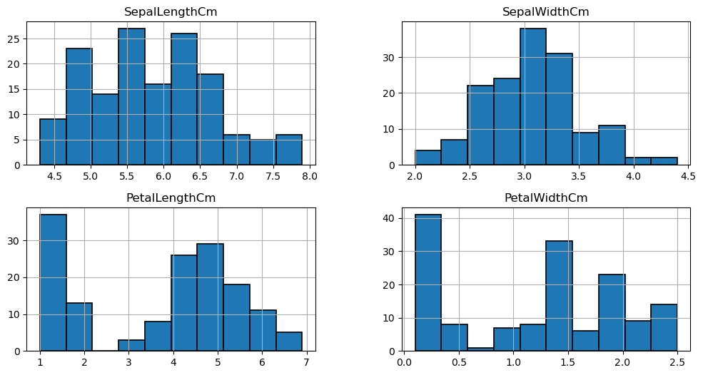
plt.figure(figsize=(15,10))
plt.subplot(2,2,1)
sns.violinplot(x='Species', y='PetalLengthCm', data=iris)
plt.subplot(2,2,2)
sns.violinplot(x='Species', y='PetalWidthCm', data=iris)
plt.subplot(2,2,3)
sns.violinplot(x='Species', y='SepalLengthCm', data=iris)
plt.subplot(2,2,4)
sns.violinplot(x='Species', y='SepalWidthCm', data=iris)
#Length와 Width가 종에 따라 어떻게 다른지 나타내는 그래프들
#violinplot은 종에 따른 길이와 너비의 밀도를 보여주는데 얇은 부분은 낮은 밀도를 나타낸다.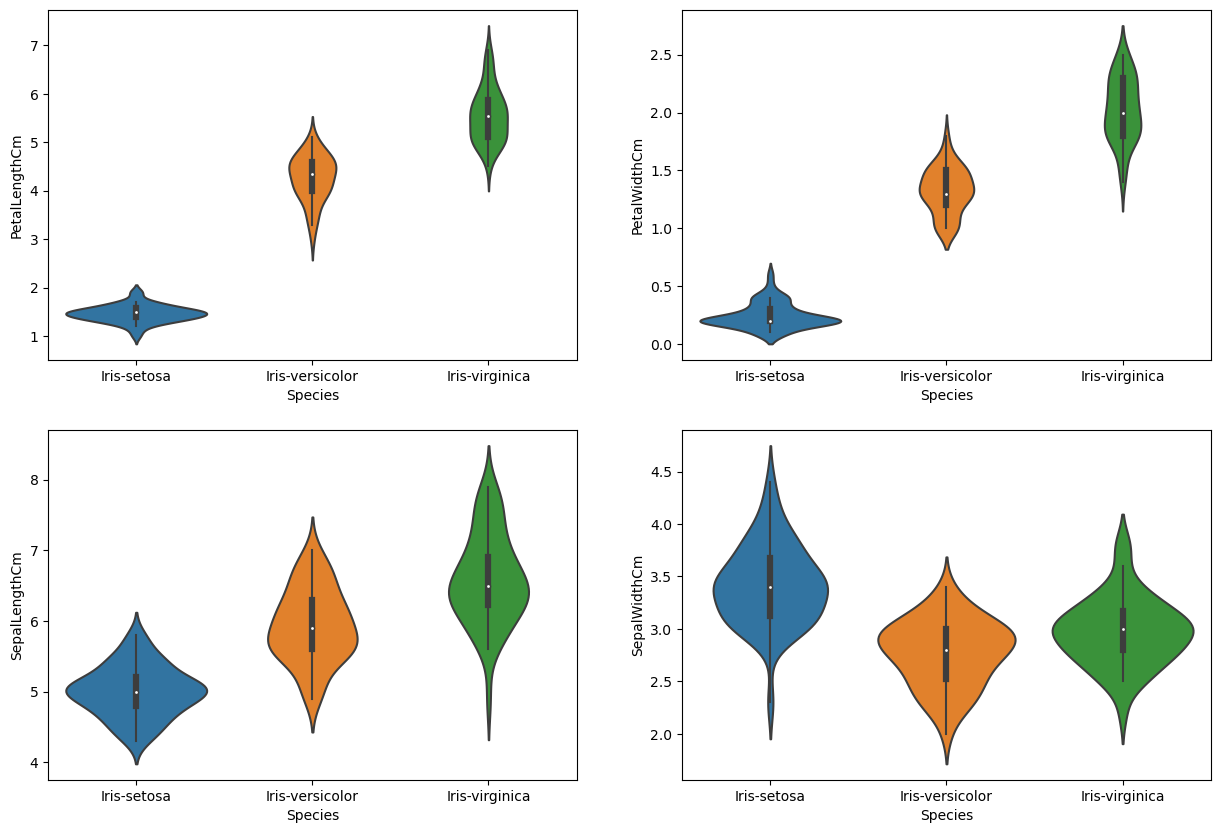
from sklearn.linear_model import LogisticRegression
from sklearn.model_selection import train_test_split
from sklearn.neighbors import KNeighborsClassifier
from sklearn import svm
from sklearn import metrics
from sklearn.tree import DecisionTreeClassifier
iris.shape
#dataset의 shape 출력(150, 5)
plt.figure(figsize=(7,4))
sns.heatmap(iris.corr(numeric_only=True), annot=True, cmap='cubehelix_r')
plt.show()
#corr는 상관관계를 계산해준다.
#많은 특성들이 높은 상관관계를 보인다면 모든 특성을 사용하여 알고리즘을 훈련하는 것은 정확도를 떨어뜨릴 것이다.
#결과
#Sepal width와 length는 상관관계가 없지만 Petal width와 length는 높은 상관관계를 보인다.
#상관관계가 없는 두 특성을 사용해서 정확도를 확인할거다
#왜 상관관계가 없는걸 사용하냐면 dataset의 다양성과 과적합 방지, 중요한 특성인지 파악하기 위해서이다.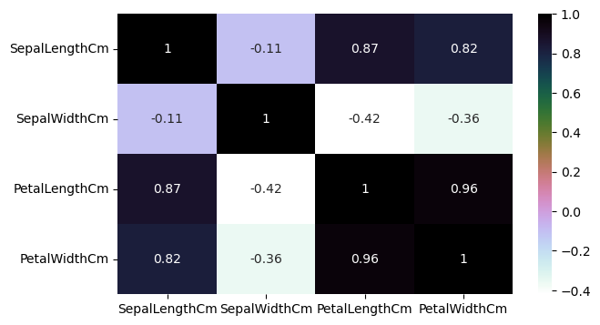
#알고리즘 적용할때는
#1. 데이터셋을 train set과 test set으로 나눈다
#2. 문제(분류, 회귀)에 맞는 알고리즘을 선택한다.
#3. train set을 알고리즘에 전달하여 훈련시킨다. 이때 fit() 사용
#4. 훈련된 알고리즘에 test set을 전달하여 결과를 예측한다. 이때 .predict() 사용
#5. 예측된 결과와 실제 출력을 모델에 전달하여 정확도를 확인한다.
train, test = train_test_split(iris, test_size=0.3)

print(train.shape)
print(test.shape)

#test set의 비율이 0.3이 되도록 나눔
#결과적으로 train 105개, test 45개로 나뉨
(105, 5)
(45, 5)
train_X = train[['SepalLengthCm', 'SepalWidthCm', 'PetalLengthCm', 'PetalWidthCm']]
train_y = train.Species
test_X = train[['SepalLengthCm', 'SepalWidthCm', 'PetalLengthCm', 'PetalWidthCm']]
test_y = train.Species
#X에는 Features를 넣고 Y에는 output 결과로 나올 data를 집어넣는다.
train_X.head(2)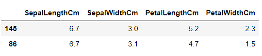
test_X.head(2)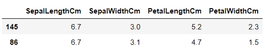
train_y.head()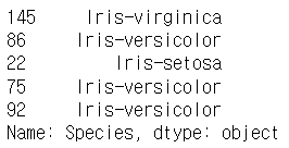
model = svm.SVC() #algorithm을 SVM으로 정했다.
model.fit(train_X, train_y) #.fit() 함수에 train 값을 넣어 train 시킨다.
prediction = model.predict(test_X) #.predict()함수에 test input 값 넣고 예측한다.
print('The accuracy of the SVM is: ', metrics.accuracy_score(prediction, test_y))
#예측한 값과 정답값을 accuracy_score에 넣고 정확도를 구한다.
#SVM의 성능은 매우 좋다
The accuracy of the SVM is: 0.9904761904761905
model = LogisticRegression(max_iter=500) #이번엔 Logistic Regression을 써보자
model.fit(train_X, train_y)
prediction = model.predict(test_X)
print('The accuracy of the LogisticRegression is: ', metrics.accuracy_score(prediction, test_y))
#max_iter를 지정하지 않으니 알고리즘이 수렴을 하지 못했다는 경고메세지가 떴다.
#경고메세지가 뜬다면 max_iter를 500이상으로 크게 설정해주자
#LogisticRegression도 성능이 좋다.
The accuracy of the LogisticRegression is: 0.9809523809523809
model = DecisionTreeClassifier() #이번엔 DecisionTreeClassifier를 써보자
model.fit(train_X, train_y)
prediction = model.predict(test_X)
print('The accuracy of the DecisionTreeClassifier is: ', metrics.accuracy_score(prediction, test_y))
#DecisionTreeClassifier도 성능이 좋다.
The accuracy of the DecisionTreeClassifier is: 1.0
model = KNeighborsClassifier(n_neighbors=3)
model.fit(train_X, train_y)
prediction = model.predict(test_X)
print('The accuracy of the KNeighborsClassifier is: ', metrics.accuracy_score(prediction, test_y))
#SciPy의 업데이트 때문에 오류가 뜨는데 크게 신경쓸 필요는 없을 것 같다.
#KNeighborsClassifier도 성능이 좋다.
The accuracy of the KNeighborsClassifier is: 0.9809523809523809
a_index=list(range(1,11))
a=pd.Series()
x=[1,2,3,4,5,6,7,8,9,10]
for i in list(range(1,11)):
    model=KNeighborsClassifier(n_neighbors=i)
    model.fit(train_X, train_y)
    prediction=model.predict(test_X)
    a=a.append(pd.Series(metrics.accuracy_score(prediction, test_y)))
plt.plot(a_index, a)
plt.xticks(x)

#n_neighbors의 값을 여러가지로 실험해봄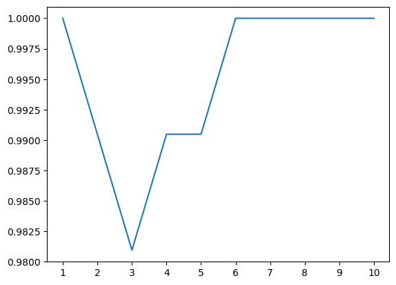
#이제 Petal과 Sepal을 따로 사용해볼것임
petal = iris[['PetalLengthCm', 'PetalWidthCm', 'Species']]
sepal = iris[['SepalLengthCm', 'SepalWidthCm', 'Species']]
train_p, test_p = train_test_split(petal, test_size=0.3, random_state=0)
train_x_p=train_p[['PetalWidthCm', 'PetalLengthCm']]
train_y_p=train_p.Species
test_x_p=test_p[['PetalWidthCm', 'PetalLengthCm']]
test_y_p=test_p.Species
train_s, test_s = train_test_split(sepal, test_size=0.3, random_state=0)
train_x_s=train_s[['SepalWidthCm', 'SepalLengthCm']]
train_y_s=train_s.Species
test_x_s=test_s[['SepalWidthCm', 'SepalLengthCm']]
test_y_s=test_s.Speciesmodel=svm.SVC()
model.fit(train_x_p, train_y_p)
prediction=model.predict(test_x_p)
print('The accuracy of the SVM using Petal is : ', metrics.accuracy_score(prediction, test_y_p))
model=svm.SVC()
model.fit(train_x_s, train_y_s)
prediction=model.predict(test_x_s)
print('The accuracy of the SVM using Sepal is : ', metrics.accuracy_score(prediction, test_y_s))The accuracy of the SVM using Petal is : 0.9777777777777777
The accuracy of the SVM using Sepal is : 0.8
model=LogisticRegression()
model.fit(train_x_p, train_y_p)
prediction=model.predict(test_x_p)
print('The accuracy of the LogisticRegression using Petal is : ', metrics.accuracy_score(prediction, test_y_p))

model=LogisticRegression()
model.fit(train_x_s, train_y_s)
prediction=model.predict(test_x_s)
print('The accuracy of the LogisticRegression using Sepal is : ', metrics.accuracy_score(prediction, test_y_s))
The accuracy of the LogisticRegression using Petal is : 0.9777777777777777
The accuracy of the LogisticRegression using Sepal is : 0.8222222222222222
model=DecisionTreeClassifier()
model.fit(train_x_p, train_y_p)
prediction=model.predict(test_x_p)
print('The accuracy of the DecisionTreeClassifier using Petal is : ', metrics.accuracy_score(prediction, test_y_p))

model=DecisionTreeClassifier()
model.fit(train_x_s, train_y_s)
prediction=model.predict(test_x_s)
print('The accuracy of the DecisionTreeClassifier using Sepal is : ', metrics.accuracy_score(prediction, test_y_s))
The accuracy of the DecisionTreeClassifier using Petal is : 0.9555555555555556
The accuracy of the DecisionTreeClassifier using Sepal is : 0.6444444444444445
model=KNeighborsClassifier(n_neighbors=3)
model.fit(train_x_p, train_y_p)
prediction=model.predict(test_x_p)
print('The accuracy of the KNeighborsClassifier using Petal is : ', metrics.accuracy_score(prediction, test_y_p))

model=KNeighborsClassifier(n_neighbors=3)
model.fit(train_x_s, train_y_s)
prediction=model.predict(test_x_s)
print('The accuracy of the KNeighborsClassifier using Sepal is : ', metrics.accuracy_score(prediction, test_y_s))
The accuracy of the KNeighborsClassifier using Petal is : 0.9777777777777777
The accuracy of the KNeighborsClassifier using Sepal is : 0.7333333333333333
#관찰 결과
#Petal을 사용하는 것이 Sepal을 사용하는 것보다 정확도가 높다
#Petal의 width와 length의 상관관계가 높았기 때문에 그런 것 같다.
참고 : Iris Dataset
